Operations research.pptx

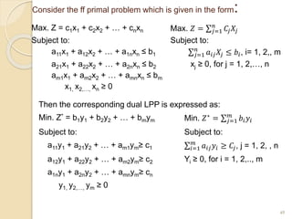
1.1 Definitions of operations research
 The British/Europeans refer to "operational research“
 The Americans refer to "operations research" but both are often
shortened to just "OR”.
 Another term which is used for this field is "management science"
("MS").
 The Americans sometimes combine the terms OR and MS
together and say "OR/MS" or "ORMS".
 Yet other terms sometimes used are "industrial engineering" ("IE")
and "decision science" ("DS").
 In recent years, there has been a move towards a standardization
upon a single term for the field, namely the term "OR".
2
Chapter One
Introduction to Operation Research

Cont’d…
 The contents and the boundaries of the OR are not yet fixed..
 Therefore, defining OR is a difficult task.
 OR is the art of winning wars without actually fighting. – Aurther
Clarke (LPP, Assignment problem,..etc).
 OR is the art of giving bad answers to problems which otherwise
have worse answers. – Thomas L. Saaty (Scarcity)
 OR is a science which deals with problem identification,
formulation, solutions & finally appropriate decision making.
 OR is the use of mathematical models, statistics & algorithm to
aid in decision-making.
 OR is concerned with scientifically deciding how to best design &
operate man-machine system usually requiring the allocation of
scare resources.
3

1.2 History of Operation Research
 OR is a relatively new discipline.
 It was in the 1930's that OR began in a systematic fashion in
the UK.
 The main origin of OR was during the Second World War
(1939-1945).
 The objective was to make the best use of limited military
resources to win the war.
 At the time of WWII , the military management in England
invited a team of scientists to study the strategic and tactical
problems related to air and land defense of the country.
 The problem attained importance b/c:
 At that time the resources available with England was very
limited and
 The objective was to win the war with available meager
resources.
4

Cont’d…
 The resources such as food, medicines, manpower etc., were required
to manage war and for the use of the population of the country.
 It was necessary to decide upon the most effective utilization of the
available resources to achieve the objective.
 It was also necessary to utilize the military resources cautiously.
 Hence, the Generals of the military invited a scientists, doctors,
mathematicians, business people, professors, engineers etc., and the
problem of resource utilization is given to them to discuss and come out
with a feasible solution.
 These specialists had a brain storming session and came out with a
method of solving the problem, which they coined the name “Linear
Programming” in 1940s by George Dantzig.
 This method worked out well in solving the war problem.
5

1.3 Operations Research Modeling Approach
1. Defining the problem and gathering data
 This procedure is crucial
 it is difficult to extract a “right” answer from the
“wrong” problem.
 Most practical problems encountered by OR teams
are initially described in a vague and imprecise way
 This step should answer the following questions:
 Who are the decision makers? ,
 What are the objectives? ,
 what are the constraints (relationships)? And
 How to collect relevant data.
7

2. Formulating a mathematical model
 After the decision maker’s problem is defined,
 the next phase is to reformulate this problem convenient for analysis
 The conventional OR approach is to construct a mathematical model to:
 represents the essence of the problem.
 Mathematical models are also idealized representations of problems
 expressed in terms of mathematical symbols and expressions.
 This step needs to define decision variables,
 The objective function (maximization/minimization), and
 The constraints (relations among decision variables).
8

3. Deriving solutions from the model
 After a mathematical model is formulated for the problem under
consideration,
 The next phase in an OR study is to develop a procedure for deriving
solutions to the problem from the model
 It is a relatively simple step, in which one of the standard algorithms of
OR is applied on a computer
 A common theme in OR is the search for an optimal, or best, solution
 Many procedures have been developed for finding such solutions for
certain kinds of problems
 Need an algorithm (systematic solution procedures).
 Conduct post-optimality analysis (Sensitivity analysis).
 What would happen to the optimal solution if different assumptions are
made?
9

4. Implementation
 Install a well-documented system for applying the model
 Include the model, solution procedure, and operating procedures for
implementation.
 A considerable number of computer programs often need to be used
and integrated
 Databases and management information systems may provide up-to-
date input for the model
 The assumptions of the model continue to be satisfied
 Need to revise or re-build models when significant deviations occur.
10

1.4 Application of Operation Research
 It provides a tool for scientific analysis and provides solution for
various business problems.
 It enables optimum allocation of scarce resources.
 It helps in minimizing waiting and servicing costs.
 It enables the management to decide when to buy and how much to
buy through the technique of inventory planning.
 It helps in evaluating situations involving uncertainty.
 It enables experimentation with models, thus eliminating the cost of
making errors while experimenting with reality.
 It allows quick and inexpensive examination of large numbers of
alternatives.
 In general, OR facilitates and improves the decision making process.
11

1.5 Limitation of Operation Research
 Magnitude of computation: In order to arrive at an optimum solution, OR
takes into account all the variables that affect the system. Hence, the
magnitude of computation is very large.
 Non-Quantifiable variables: OR can give an optimum solution to a problem
if all the variables are quantified. But, all variables in a system cannot be
quantified.
 Time and Cost: To implement OR in an organization, it consumes more time
and cost. If the basic decision variables change, OR becomes too costly for
an organization to handle it.
 Implementation of OR: Implementation of OR may lead to human resource
problems. The psychology of employees should be considered.
 Distance b/n Manager and OR Specialist: Managers may not be having a
complete overview of OR techniques and has to depend upon an OR
Specialist. Only if good link is established OR can be a success.
12

Chapter two: Linear programming
2.1 Basic concepts in linear programming
 Linear Programming is one of the most versatile, powerful and useful
techniques for making managerial decisions.
 It is used for solving broad range of problems arising in business,
government, industry, hospitals, libraries, etc.
 If a real-world problem can be represented accurately by the
mathematical equations of a linear program, the method will find the
best solution to the problem.
 The term linear implies the condition of proportionality and additivity.
 Programming is the process of finding the maximum or minimum
value subjected to various constraints.
 LP is a mathematical technique for finding optimal solutions to
problems that can be expressed using linear equations & inequalities
13

Cont’d…
 Purpose: optimal allocation of scarce
resources (labor, material, machine, time,
warehouse, space, capital, etc) among
competing products/activities
 It is often necessary to optimize a
profit/cost function
 A linear program consists:
® Set of variables,
® A linear objective function indicating the
contribution of each variable and
® A set of linear constraints describing the
limits on the values of the variables.
 LP problem must have
the ff ppties:
 The r/ship b/n variables
& constraints must be
linear.
 The model must have:
 An objective function.
 Structural constraints.
 Non-negativity constraint.
14

2.2 Formulation of linear programming problems
 Objective function: the goal or objective of a management, stated
as intent to maximize or to minimize some important quantity such as
profits or costs.
 Z= 𝑗=1
𝑛
CjXj
 Cj = the objective function coefficient
 Xj = the jth decision variable
 Constraints: it indicate limitations on the resources (production
capacity, manpower, time, space or machinery), which are to be
allocated among various decision variables.
 It can be expressed as linear equalities or inequalities arising out of
practical limitations.
 Subject to (st) 𝑗=1
𝑛
aijX j ≤ bi; Xi= the ith decision variable,
 Aij = the coefficient of xi in constraint (resource use); bi = RHS 15

 The constants (the coefficients & RHS) in the constraints
and the objective function are called the parameters of the
model.
 Decision variables: the set of quantities that need to be
determined in order to solve the problem
 The variables represent the amount of a resource to use/
the level of some activity.
 Non-negativity constraints: the variables of linear
programs must always take non-negative values (i.e., they
must be greater than or equal to zero).
16

Cont’d…
 In formulating the LPP as a mathematical model, we
shall follow the following four steps:
1.Identify the decision variables and assign symbols to
them (eg x, y, z,. . .or x1, x2, x3, . . .
2.Identify the objective function and express it in terms of
the decision variables.
3.Identify the set of constraints and express them in terms
of inequalities involving the decision variables.
4.Add the non-negativity constraints
17

2.3Assumptions of linear programming
1. Proportionality assumption: It states that the contribution of
each activity to the value of the objective function Z is proportional to
the level of the activity Xj, as represented by the CjXj term in the
objective function.
 Similarly, the resource consumption of each activity in each
functional constraint is proportional to the level of the activity Xj,
as represented by the aijXj term in the constraint.
2. Additivity assumption: States that every function in a LPP is the
sum of the individual contributions of the respective activities.
3. Divisibility assumption: States that the numerical values of the
decision variables are continuous and not limited to integers.
In other words, fractional values of the decision variables must be
permissible in obtaining optimal solution. 18

Cont’d…
4. Certainty assumption: The value assigned to each
parameter of a LPP is assumed to be a known constant
(never change through time).
However, in real applications, the certainty assumption is
seldom satisfied precisely.
5. Finiteness: An LP model assumes that a finite (limited)
number of choices (alternatives) are available to the decision-
maker and that the decision variables are interrelated and
non-negative.
6. Optimality: In LP, the optimal solution always occurs at the
corner point of the set of feasible solutions.
19

2.3 Methods of solving LP
 Linear Programming is a method of solving the type of
problem in which two or more candidates or activities are
competing to utilize the available limited resources, with a
view to optimize the objective function of the problem.
 The objective may be:
 to maximize the returns or
 to minimize the costs.
 The various methods available to solve the problem are:
1. Graphical method
2. Simplex method
3. Software (R, Excel, POM-QM etc)
20

2.3.1The graphical method
 The Graphical Method is used to solve LPP when we have two
decision variables.
 Hence , it is limited to two variable problems.
 The inequalities are considered to be equations b/c difficult to draw a
graph for inequality.
 The characteristics of Graphical method are:
 The method is used to solve the two decision variables LPP problems
 It requires high imagination for three or more decision variables to
identify the solution area.
 Always, the solution to the problem lies in first quadrant b/c Xi ≥ 0.
 This method provides a basis for understanding the other methods of
solution. 21

Cont’d…
To sole LPP graphically, the following steps are necessary:
1. Formulate mathematical model of linear programming
2. Convert constraint inequalities into equalities
3. Draw the graph by intercept (graphs of constraints) & shade
4. Identify the feasible region of the solution which satisfies all
constrains.
5. Identify the corner points in the feasible region
6. Identify the optimal point
7. Interpret the result
Graphical LP is a two-dimensional model.
Maximization problem: maximize z with inequalities of constraints
in < form.
Maximization.docx
22

Example: consider two models of color TV sets; model A and B,
are produced by a company to maximize profit. The profit realized is
$300 from A and $250 from set B. The limitations are
A. Availability of only 40hrs of labor each day in the production
department.
B. A daily availability of only 45 hrs on machine time
C. Ability to sale 12 set of model A. (Products < customers’ demand)
How many sets of each model will be produced each day so that the
total profit will be as large as possible?
Resources used per unit
Constraints Model a model b
(x1) (x2)
Maximum available hrs.
Labor hr. 2 1 40
Machine hr. 1 3 45
Marketing 1 0 12
Profit $300
$250 23

Exercise
An aluminum plant produces two types of aluminum:
type I and type II. Type I takes 6 hours for melting, 3
hours for rolling, and 1 hour for cutting. Type II takes
2 hours for melting, 5 hours for rolling, and 4 hours
for cutting. The plant has 36 hours of melting time
available, 30 hours of rolling time, and 20 hours of
cutting time. The profit margin is $10 and $8 per unit
for type I and type II, respectively. How many
quantities of each type have to be produced to
obtain the maximum profit?
24

Minimization problem
==>minimize z with inequalities of constraints in > form
Example: suppose that a machine shop has two different types of
machines; machine 1 and machine 2, which can be used to make a single
product .These machines vary in the amount of product produced per hr., in
the amount of labor used and in the cost of operation.
How much should we utilize each machine in order to minimize the total
costs and still meets the requirement?
resource used
Constraints machine 1 (x1) machine (x2) minimum
required hours
Product produced/hr 20 15 100
Labor/hr 2 3 15
Operation cost $25 $30
Minimization.docx 25

Special cases in graphics methods
1. Redundant constraint
 If a constraint doesn’t form part of the boundary making the feasible
region of the problem when plotted on a graph.
2. Multiple optimal solutions
 We have unlimited number of optimal solution without increasing or
decreasing the objective function.
 Multiple optimal solutions provide more choices for management to
reach their objectives.
3. Infeasible solution
 But the graphs of the constraints don’t form feasible region
4. Unbounded solution it is a solution whose objective function is
infinite (The objective function has no lower and upper limit).
26

2.4.2 Simplex method
 Simplex method is most powerful method.
 It deals with iterative process, which consists of first designing a basic
feasible solution or a programme and proceed towards the optimal
solution and
 Testing each feasible solution for optimality to know whether the solution
on hand is optimal or not.
 If not an optimal solution, redesign the programme, and test for
optimality until the test confirms Optimality.
 Hence we can say that the simplex method depends on two concepts
known as feasibility and optimality.
 The iterative steps of the simplex method are repeated until a finite
optimal solution, if exists, is found.
 If no optimal solution, the method indicates that no finite solution exists.
27

 The simplex method is an ITERATIVE or “step by step” method that
moves automatically from one basic feasible solution to another
basic feasible solution improving the situation each time until the
optimal solution is reached
 Maximization problems
◦ Maximize Z with inequalities of constraints in “< “form
 Example: Solve the problem using the simplex method
Max.Z=300x1 +250x2
Subject to: 2x1 + x2 < 40 (Labor)
x1+3x2 < 45 (Machine)
x1< 12 (Marketing)
x1, x2> 0
28
Cont’d…

Cont’d…
 Solution
 Step 1: Formulate LPP Model
 Step 2: Standardize the problem: convert constraint inequality into
equality form by introducing Slack variable.
 Slack Variables are added to the left hand side of a < constraint to
covert the constraint inequality in to equality.
 Slack variable shows unused resource.
 Slack variables represent unused resource or idle capacity.
 Slack variables are added to the objective function with zero
coefficients.
 Let that s1, s2, and s3 are unused labor, machine and marketing hrs,
respectively.
29

Cont’d…
 Step 3: Obtain the initial simplex tableau
 In constructing the initial simplex tableau, the optimal solution begins at the
origin. Indicating that nothing can be produced i.e. x1 =0 and x2=0
 n-m variables set equal to zero (NBVs): BVs vs NBVs
 ==>2x1+x2+ s1 +0 s2+ 0 s3= 40 ==>x1+3x2+0 s1 + s2+ 0 s3= 45
 2(0) +0+ s1 +0 s2+ 0 s3= 40 0 +3(0)+0s1 + s2+ 0 s3= 45
 s1= 40 – Unused labor hrs. s2= 45 – Unused machine hrs.
 ==>x1+0s1 +0s2+ s3= 12
 0 +0s1 +0 s2+ s3= 12
 s3= 12 – Unused Marketing hrs.
 Therefore, Max.Z=300x1 +250x2 + 0 s1 +0 s2+ 0 s3 =300(0) +250(0) +
0(40) +0(45) + 0(12) = 0
31

 Step 4: Construct the initial simplex
tableau
 Initial simplex tableau
32
Cj 300 250 0 0 0
BV X1 X2 S1 S2 S3 Q
0 S1 2 1 1 0 0 40
0 S2 1 3 0 1 0 45
0 S3 1 0 0 0 1 12
Zj 0 0 0 0 0 0
Cj - Zj 300 250 0 0 0

 Step 5: Choose the “incoming” or “entering” variables
 The entering variable is the variable that has the most positive
value in the Cj – Zj row (Refer step 4 simplex tableau)
 Step 6: Choose the “leaving “or “outgoing” variable
 Note: The row with the minimum or lowest positive (non-negative)
replacement ratio shows the variable to leave the solution.
 Note: RR>0
 Repeat step 4-6 until optimal solution is reached.
 2nd simplex tableau.docx
33
Replacement Ratio (RR) = Solution Quantity (Q) (RHS)
Corresponding values in pivot column

 Since all the Cj - Zj< 0 optimal solution is reached at.
 Therefore, X1=12, X2=11, S1=5 and Max Z=6350
34
Cj 300 250 0 0 0
BV X1 X2 S1 S2 S3 Q
0 S1 0 0 1 -1/3 -5/3 5
250 X2 0 1 0 1/3 -1/3 11
300 X1 1 0 0 0 1 12
Zj 300 250 0 250/3 650/3 6350
Cj - Zj
0 0 0 -250/3 -
650/3

 Minimization problems
◦ Minimize Z with inequalities of constraints in “> “form
 There are two methods to solve minimization LP problems:
 1. Big M-method
◦ Using surplus and artificial variables
 2. Conversion method
◦ Minimization by maximizing the dual
 Surplus Variables are inserted in a greater than or equal to
constraint to create equality.
 Surplus variable is subtracted from a > constraint in the process of
converting the constraint to standard form.
 Artificial variable is a variable that has no meaning in a physical
sense but acts as a tool to create an initial feasible LP solution.
35

Big M-method /Charnes Penalty Method/
 If objective function Z is to be minimized, then a very large positive price
(called penalty) is assigned to each artificial variable.
 If Z is to be maximized, then a very large negative price is assigned to
each of these variables.
 Following are the characteristics of Big-M Method:
 High penalty cost (or profit) is assumed as M
 M is assigned to artificial variable A in the objective function Z.
 Big-M method can be applied to minimization & maximization problems
 Coefficient of slack/surplus takes zero values in the objective function Z
 For minimization problem, the incoming variable corresponds to the
highest negative value of Cj-Zj row
36

Example: MinZ=25x1 +30x2
Subject to:
20x1+15x2 > 100
2x1+ 3x2 > 15
x1, x2> 0
Solution: Step 1 Standardize the problem
Minimize Z=25x1 +30x2 +0s1+0s2 +MA1+MA2
Subject to:
20x1+15x2- s1+A1 = 100
2x1+ 3x2 –s2+A2 = 15
x1, x2 , s1, s2 ,A1 ,A2 > 0
Step 2: Initial simplex tableau
The initial basic feasible solution is obtained by setting x1= x2= s1=
s2=0 ==>20(0) +15(0) - 0+A1 = 100 ==> A1 = 100
x1= x2= s2=0==>0(0)+3(0) - 0+A2 =15==> A2 = 15
The number of basic variables?
37

 Initial simplex tableau
 Once an artificial variable has left the basis, it has served its
purpose and can therefore be removed from the simplex tableau
38
Cj 25 30 0 0 M M
BV X1 X2 S1 S2 A1 A2 Q
M A1 20 15 -1 0 1 0 100
M A2 2 3 0 -1 0 1 15
Zj 22M 18M -M -M M M 115 M
Cj - Zj 25 -22M 30- 18M M M 0 0

Revised simplex tableau
Cj - Zj> 0==>Optimal solution is reached
X1=5/2
X2=10/3 and MinZ=162.5
40
Cj 25 30 0 0
SV X1 X2 S1 S2 Q
25 X1 1 0 -1/10 1/2 5/2
30 X2 0 1 1/15 -2/3 10/3
Zj 25 30 -1/2 -15/2 162.5
Cj - Zj
0 0 1/2
15/2

Exercise
On a chicken farm, the poultry is given a healthy diet
to gain weight. The chickens have to consume a
minimum of 15 units of Substance A and another 20
units of Substance B. In the market there are only
two classes of compounds: Type X, with a
composition of one unit of A to five units of B, and
another type, Y, with a composition of 3 units of A to 4
units of B. The price of Type X is $10 and Type Y,
$30. What are the quantities of each type of
compound that have to be purchased to cover the
needs of the diet with a minimum cost?
42

Special cases in simplex method
 Mixed constraint: the existence of ≤ (Slack) , ≥ (Surplus +
Artificial) and = ( Artificial) signs in the constraint equation
/inequality.
E.g.
Max z=6x1 +8x2
St: x2+s1 =4
6x1+ 2x2 -s2 +a2
x1, x2> 0
 Two incoming variable: two variables have the same most +ve / -
ve cj-zj value
 DV Vs DV……arbitrary selection
 DV vs Slack/Surplus…..Selection DV
 Slack vs Slack or Surplus vs Surplus…Arbitrary.
 Infeasibility: exists when an artificial variable appears in the
solution mix (OS).
 Unbounded solution: no leaving variable b/c the RR turnout to be
–ve / undefined.
 Degeneracy: two variables have the same minimum RR
 Multiple optimal solution: the Cj-Zj value of non-basic variable/s is
/are zero.
43

Chapter three: Duality and sensitivity analysis
3.1 Duality and its essence
 Duality is a property of the simplex method that adds further versatility to
the general LP model.
 The term dual indicates that there are two ways of looking at each
problem
 Associated with every LPP, there is another intimately related LPP
 The original LPP is called the primal problem
 the corresponding intimately related problem is called its dual problem
 Both of them originate from the same data
 When the primal is solved, its associated dual is also solved
simultaneously.
 Dual problem’s variables provide useful information about the primal
problem.
44

Consider the ff primal problem which is given in the form:
Max. Z = c1x1 + c2x2 + … + cnxn Max. 𝑍 = 𝑗=1
𝑛
𝐶𝑗𝑋𝑗
Subject to: Subject to:
a11x1 + a12x2 + … + a1nxn ≤ b1 𝑗=1
𝑛
𝑎𝑖𝑗𝑋𝑗 ≤ 𝑏𝑖, i= 1, 2,, m
a21x1 + a22x2 + … + a2nxn ≤ b2 xj ≥ 0, for j = 1, 2,…, n
am1x1 + am2x2 + … + amnxn ≤ bm
x1, x2,…, xn ≥ 0
45
Then the corresponding dual LPP is expressed as:
Min. Z* = b1y1 + b2y2 + … + bmym Min. 𝑍∗ = 𝑗=1
𝑚
𝑏𝑖𝑦𝑖
a11y1 + a21y2 + … + am1ym≥ c1 𝑖=1
𝑚
𝑎𝑖𝑗𝑦𝑖 ≥ 𝐶𝑗, j = 1, 2, , n
a12y1 + a22y2 + … + am2ym≥ c2 Yi ≥ 0, for i = 1, 2,.., m
a1ny1 + a2ny2 + … + amnym≥ cn
y1, y2,…, ym ≥ 0

3.2 Primal-Dual Relationship
 The number of variables in the dual = the number of constraints in
the primal problem.
 The number of constraints in the dual = the number of variables in
the primal problem.
 Coefficients (Cj) of the objective function in the dual come from the
RHS of the primal problem.
 If the primal is a maximization, the dual is a minimization
 The coefficients for the first constraint in the dual problem are the
coefficients of the first variable in the constraints for primal problem
 The RHS of the dual constraints come from the objective function
coefficients in the primal problem.
 The dual of the dual problem is the original LPP itself.
46

Let us show these through illustrative example:
Primal Dual
Max. Z = 6x1 + 4x2 Min. Z* = 12y1 + 20y2 + 24y3
4x1 + x2 ≤ 12 4y1 + 9y2 + 3y3 ≥ 6
9x1 + 2x2 ≤ 20 y1 + 2y2 + 5y3 ≥ 4
3x1 + 5x2 ≤ 24 y1, y2, y3 ≥ 0
x1, x2 ≥ 0
47
Depending on the above example:
Primal Dual
Maximization Minimization
Objective function is written as z In dual as z*
Two variables Two constraints
Three constraints Three variables
6 and 4 are Cj of the objective function 6 and 4 are RHSs
The coefficients of constraints
4
9
3
1
2
5
The coefficients of constraints
4
1
9
2
3
5
≤ signs of constraints ≥signs of constraints



Duality for Mixed Constraints
 In practice, many linear programs contain some constraints of the
≤, ≥, and = types.
 Transformation techniques can be applied to convert any "mixed“
constraints to standard forms i.e.
 For maximization problem: all the signs of the constraints should
be written in ≤ and
 For minimization, ≥
48
Max. Z = 6X1 + 10X2
Subject to:
4X1 + X2 ≤ 12 9X1 + 2X2 ≥ 20 ( multiply both side by -1)
9X1 + 2X2 = 20 -9X1 - 2X2 ≤ -20
3X1 + 5X2 ≥ 24 9X1 + 2X2 ≤ 20
X1, X2 ≥ 0 Multiply both sides by -1 -3X1 - 5X2 ≤ -
24

The primal problem is standardized just like this:
49
Max. Z = 6X1 + 10X2
Subject to:
4X1 + X2 ≤ 12
-9X1 - 2X2 ≤ - 20
9X1 + 2X2 ≤ 20
-3X1 - 5X2 ≤ -24
X1, X2 ≥ 0
The dual problem is as follows:
Minz* =12Y1 - 20Y2 + 20Y3 - 24Y4
Subject to:
4Y1 - 9Y2 + 9Y3 - 3Y4 ≥ 6
Y1 - 2Y2 + 2Y3 - 5Y3 ≥ 10
Y1, Y2, Y3, Y4 ≥ 0

Solution of Primal and Dual Problem
50
 Solution of primal problem:
 Introducing the slack variables, the problem becomes:
 Max. Z = 20x1 + 50x2 + 0s1 + 0s2
 Subject to:
 5x1 + 4x2 + s1 + 0s2 = 20
 3x1 + 5x2 + 0s1 + s2 = 15
 x1, x2, s1, s2 ≥ 0
 The initial simplex tableau is: Primal problem.docx
Primal problem
Max. Z = 20x1 + 50x2
Subject to:
5x1 + 4x2 ≤ 20
3x1 + 5x2 ≤ 15
x1, x2 ≥ 0
Solve both the
primal and dual
of the following
LPP and
observe their
relation
Dual problem
Min. Z* = 20y1 + 15y2
Subject to:
5y1 + 3y2 ≥ 20
4y1 + 5y2 ≥ 50
y1, y2 ≥ 0
Solution
X1 = 0
X2 = 3 and
MAXZ = 150

Solution of dual problem
 Introducing the surplus variables, the problem becomes:
 Min. Z* = 20Y1 + 15Y2 + 0S1 + 0S2 + MA1 + MA2
 Subject to:
5Y1 + 3Y2 - S1 + 0S2 + A1 + 0A2 = 20
4Y1 + 5Y2 + 0S1 - S2 + 0A2 + A2 = 50
Y1, Y2, S1, S2 ≥ 0
Dual problem.docx
51
Y1 = 0 , Y2 = 10 and MinZ* = 150
Interpretation:
The solution indicates that the value of the objective function will be
increased by 10 unit for a unit change in RHS of the 2nd constraint
Dual solution is also called:
 Shadow price or
 Marginal value of resources (the worth of one unit of the
resource at optimal point)
 LPP......with Excel Solver.mp4

Sensitivity analysis
 The method of evaluating the degree to which the present optimal
solution is continued as optimal is called sensitivity analysis.
 It is concerned with the study of change in the optimal solution of a
LPP with changes in parameters.
 It deals with how the optimal solution is affected by changes
 In this case, we are going to determine the range (both lower and
upper) over which the linear programming model parameters can
change without affecting the current optimal solution.
 Sensitivity analysis means determining effects of changes in
parameters on the solution.
 It is also called
 What if analysis,
 Post optimality analysis, etc
52

 Sensitivity analysis (or post-optimality analysis) is used to determine
how the optimal solution is affected by changes, within specified
ranges, in:
the objective function coefficients
the right-hand side (RHS) values
 Sensitivity analysis is important to the manager who must operate in
a dynamic environment with imprecise estimates of the coefficients.
 Sensitivity analysis allows the manager to ask certain what-if
questions about the problem.
53

Cont’d..
 Sensitivity analysis deals with:
1. Changes in Cj of basic and non-basic variables
 1.1 Change in coefficient Cj of non-basic variable
 Among the variables included in the LPP, some are non-basic
variables (n-m variables)
 Change in coefficient Cj of non-basic variable:
 It doesn’t affect any of cj values of basic variables.
 It doesn’t affect any of zj values.
 It affects ∆j values.
 It does not affect value of the objective function
54

Cont’d…
55
Example: max. Z = 2x1 + 3x2
subject to:
4x1 + 3x2 ≤ 18
5x1 + 2x2 ≤ 19
x1, x2 ≥ 0
From the final simplex table, we
can conclude that
 X1 and S1 are non-basic
variables; whereas,
 X2 and S2 are basic variables.

Cont’d…
 C1 = 2 is the coefficient of non-basic variable x1, and
 assume that c1 is subject to change by ∆c1.
 Where ∆𝐶1 = 𝐶1
′
− 𝐶1. As you remember to maintain the optimality
condition all the elements in the ∆j row should be all non-negative.
 In this case:
56
∆j1 ≥ 0 ∆𝐶1 ≤ 2
𝑍1 − 𝐶1
′
≥ 0𝐶1
′
− 𝐶1 ≤ 2
𝑍1 − (𝐶1 + ∆𝐶1) ≥ 0𝐶1
′
− 2 ≤ 2
𝑍1 − 𝐶1 − ∆𝐶1 ≥ 0𝐶1
′
≤ 4
4 − 2 − ∆𝐶1 ≥ 0(−∞, 4]
−∆𝐶1 ≥ −2
∆𝐶1 ≤ 2
(−∞, 2)
Therefore, the range over which the parameter (c1) can change
without affecting the current optimal solution x1 = 0 and x2 = 6 is
−∞, 4 .

1.2 Change in coefficient Cj of basic variable xj
 Change in the coefficients of basic variable
 affect zj,
 affect ∆j and
 affect the value of objective function.
 For the above table X2 is basic variable, and
 suppose C2 is changed by ∆C2 i.e. 𝐶2
′
= 3 + ∆𝐶2.
57
Cj 2 3 + ∆c2 0 0
Cj Bv X1 X2 S1 S2 Xb
3+∆c2 X2 4/3 1 1/3 0 6
0 S2 7/3 0 -2/3 1 7
Zj 4 + 4
3 ∆𝐶2
3 + ∆c2 1 + 1
3 ∆𝐶2
0 18+6∆c2
∆j 2 + 4
3 ∆𝐶2
0 1 + 1
3 ∆𝐶2
0

 The current solution will be optimal so long as all the
∆j values are non-negative.
 Therefore:
58
2 + 4
3 ∆𝐶2 ≥ 01 + 1
3 ∆𝐶2 ≥ 0
∆𝐶2 ≥ − 3
2 ∆𝐶2 ≥ −3
Their intersection is ∆𝐶2 ≥ − 3
2 or [ ∞).
Therefore, the range over which the parameter 𝑪𝟐
′
can
change without affecting the current optimal solution
X1 = 0 and X2 = 6 is [3
2 , ∞).
C’2 – C2 ≥ ∆𝐶2

2. The variation in the RHS constants (bi’s)
2.1 Sensitivity of bi’s of fully utilized resources
If resources are fully utilized,
 a non-zero shadow price will appear in the ∆j row
corresponding to slack or surplus variables in the
primal problem of the optimal solution tableau.
 The value indicates that by how much the value of
objective function will change for one additional
unit of the corresponding resource (fully utilized).
59

Cj 2 3 0 0
Cj Bv X1 X2 S1 S2 Xb
3 X2 4/3 1 1/3 0 6
0 S2 7/3 0 -
2/3
1` 7
Zj 4 3 1 0 18
∆j 2 0 1 0
 Suppose the first (fully utilized)
resource increase by one unit
and become 19 (i.e., b1 = 19).
 The new solution would be:
60
The first resource is fully
utilized.
Therefore, its shadow price is
1.
This implies that
 if we add one additional unit
of the first resource,
 the value of z will increase
by 1 unit.
𝑋𝑏 = 𝐵−1𝑏𝑛
𝐵−1
Inverse of x2 and s2 coefficients
in the standardized model (Basic
variables of LPP)
=
1
3 0
−2
3 1
*
18 + ∆𝑏1
19
=
1
3 0
−2
3 1
*
18 + 1
19
=
1
3 0
−2
3 1
*
19
19
𝑋2
𝑆2
=
19
3
19
3

 The new solution would be
X1 = 0,
X2 = 19/3 and
MaxZ = 19.
 When there is a change in the value of bi’s of fully utilized
resources, the current optimal solution will change by the
value of ∆j of slack/surplus variables.
2.1 Sensitivity of bi’s (which is not fully utilized)
 If resources are not fully utilized,
 a zero shadow price will appear in the ∆j row
 The value indicates that the value of objective function will not
change for any additional unit of that resource.
61

Exercise
MaxZ = 8X1 + 5X2
subject to
2X1 + X2 ≤ 1200
3X1 + 4X2 ≤ 2400
X1 + X2 ≤ 800
X1 + X2 ≤ 450
X1, X2 ≥ 0
Questions
a) Test the change in Cj of basic and non-basic
variables
b) Find the new optimal solution if the RHS of fully
utilized resource is increased by one unit
62

CHAPTER FOUR
THE TRANSPORTATION PROBLEMS
4.1Transportation problem Model
 LP is applicable in the physical distribution of goods from several
supply centers to several demand centers
 It is easy to express a transportation problem mathematically in
terms of an LP model
 However, since it involves a large number of variables and
constraints, it takes a long time to solve it.
 Therefore, transportation algorithms have been developed for this
purpose.
 The structure of transportation problem involves a large number of
shipping routes from several supply origins to several demand
destinations. 63

Cont’d…
 The objective of transportation problem minimalizing transportation cost.
 The places where goods originate from are called the sources or the
origins and places where they are to be shipped are called the
destinations.
 The transportation algorithm applies to minimize the total cost of
transporting a homogenous commodity.
 General transportation problem model:
 A transportation problem model, which has ‘m’ (origins and ‘n’
destinations provides a framework for presenting all relevant data.
These are:
 Quantity supply of each origin
 Quantity demand of each destination
 Unit transportation cost from each origin to each destination
64

Transportation model and general LPP
 Similarities
 Both have objective function, linear objective function and non
- negativity constraints.
 Both can be solved by simplex method. In transportation
model it is laborious.
 Differences
 Transportation model is a minimization model; where as
general LPP may be of maximization type or minimization
type.
 The resources, for which, the structural constraints are built
up is homogeneous in transportation model; where as in
general LPP they are different.
 The transportation problem is solved by transportation
algorithm; whereas, the general LPP is solved by graphical
and simplex methods.
65

Cont’d…
 The transportation algorithm requires the assumptions
that:
 All goods are homogeneous, so that any origin is capable
of supplying to any destination.
 Transportation costs are a linear function of (or directly
proportional to) the quantity shipped over any route.
 Each source has a fixed supply of units, where this entire
supply must be distributed to the destinations.
 Similarly, each destination has a fixed demand for units,
where this entire demand must be received from the 66

Destination
Source
(origins)
To
From
D1 D2 … Dn Total
Supply
S1 X11 C11 X12 C12 … X1n C
1
n
SS1
S2 X21 C21 X22 C22 … X2n C
2
n
SS2
: : : : : :
Sm Xm1 Cm1 Xm2 Cm2 … Xmn C
m
n
SSm
Total Demand dd1 dd2 … ddm
𝑆𝑆
67

Cont’d…
 Before applying the transportation algorithm to solve a specific
problem, it is necessary to satisfy the following conditions:
 Supply and requirement must be expressed in the same unit.
 Total supply must be equal to total demand, i.e., 𝑖=1
𝑚
𝑆𝑆𝑖 = 𝑗=1
𝑛
𝑑𝑑𝑗=
feasible solutions property
 This is called rim condition (𝒎 + 𝒏 − 𝟏 = BVs).
 The problem satisfied in this condition is called balanced
transportation problem
 The condition supply equals demand is the necessary and sufficient
condition for the existence of the feasible solution for the
transportation problem.
69

Cont’d…
70
 Degeneracy: An initial basic feasible solution is degenerate if m
+ n – 1 is not equal to the number of cells to which allocations
made.
 There are three pertinent cases in transportation problems.
These are:
 Balanced case: a case where total supply equals total demand
(DD = SS)
 Unbalanced transportation problem when TSS>TDD: balanced
by introducing dummy receiver
 Unbalanced transportation problem when TDD > TSS: balanced
by introducing dummy supplier
 Case 2 and case 3 are called special cases in transportation
problem.

4.2 Methods of Solving Transportation Problem
1. North West Corner method
 The method starts at the northwest-corner cell (route) of the
tableau (variable X11).
 Step 1: Allocate as much as possible to the selected cell, and
adjust the associated amounts of supply and demand by
subtracting the allocated amount.
 Step 2: Cross out the row or column with zero supply or
demand to indicate that no further assignments can be made
in that row or column.
 Step 3: If exactly one row or column is left uncrossed out,
stop. Otherwise, move to the cell to the right if a column has
just been crossed out or below if a row has been crossed out.
Go to step 1.
 Step 4: Make sure that all the rim conditions are satisfied and
(𝑚 + 𝑛 − 1) cells are allocated.
71

 Let us consider an example at this juncture to illustrate the
application of NWC rule
 The total cost of transportation = (65 × 5) + (5 × 6) + (30 × 2)
+ (7 × 5) + (43× 4) = 325 + 30 + 60 + 35 + 172 = 622.
73
To
From
W1 W2 W3 Total
Supply
S1 65 5 5 6 X13 7 70
S2 X21 4 30 2 X23 5 30
S3 X31 1 7 5 43 4 50
Total Demand 65 42 43 150
150

2. Least-Cost Method
 Steps in Least-Cost Method:
 Step 1: Determine the least cost among all the rows of the
transportation table.
 Step 2: Identify the row and allocate the maximum feasible
quantity in the cell corresponding to the least cost in the row.
Then eliminate that row (column) when an allocation is made.
 Step 3: Repeat steps 1 and 2 for the reduced transportation
table until all the available quantities are distributed to the
required places.
 Step 4: Make sure that all the rim conditions are satisfied and
(𝑚 + 𝑛 − 1) cells are allocated.
74

 Solve it using least cost method
 The total cost of transportation = (15 x 5) + (12 x 6) + (43 x 7) + (30
x 2) + (50 x 1) = 558
75
To
From
W1 W2 W3 Total Supply
S1 15 5 12 6 43 7 70
S2 4 30 2 5 30
S3 50 1 5 4 50
150

3.Vogel Approximation Method
 Step 1: For each row (column), determine a penalty measure by
subtracting the smallest unit cost from the next smallest unit cost.
 Step 2: Identify the row or column with the largest penalty. Allocate as
much as possible to the variable with the least unit cost in the
selected row
 Step 3: (a) If exactly one row or column with zero supply or demand
remains uncrossed out, stop.
 (b) If one row (column) with positive supply (demand) remains
uncrossed out, determine the basic variables in the row (column) by
the least-cost method. Stop.
 (c) If all the uncrossed out rows and columns have (remaining) zero
supply and demand, determine the zero basic variables by the least-
cost method. Stop.
 (d) Otherwise, go to step 1.
 Step 4: Make sure that all the rim conditions are satisfied and (𝑚 +
𝑛 − 1) cells are allocated.
76

 Solve using Vogel's Approximation Method
 The total cost of transportation = (15× 5) + (50× 1) + (12 × 6) + (30×
2) + (43× 7) = 558
 Tips
 Equal demand and supply for specific cell
 The same penalty measure and / least cost:
 Maximum capacity in each cell governs the allocation,
otherwise arbitrary allocation
77
To
From W1 W2 W3
Total Supply
S1 5 6 7 70
S2 4 2 5 30
S3 1 5 4 50
150

Exercise
Allocate the given transportation problem using VAM
To
From W1 W2 W3
Total Supply
S1 5 7 8 70
S2 4 4 6 30
S3 6 7 7 50
150
78

4.3 Special cases in transportation problem
 Unbalanced case: (SS > DD)
 It indicates unused supply capacity.
 How to balance?
 Dummy receiver.
 Unbalanced case: (SS < DD)
 It shows unmet demand.
 How to balance?
 Dummy supplier.
79

Unbalanced case: (SS > DD)
80
 We can convert this unbalanced case into
balanced as follows
To
From
W1 W2 W3 Total
Supply
S1 5 6 7 70
S2 4 2 5 30
S3 1 5 4 50
Total Demand 65 42 33

Unbalanced case: (SS < DD)
 We can convert this unbalanced case into
balanced as follows
81
To
From
W1 W2 W3 Total
Supply
S1 5 6 7 70
S2 4 2 5 20
S3 1 5 4 50
Total Demand 65 42 43

Tips
Equal demand and supply for specific
cell
The same penalty measure and least
cost:
Maximum capacity in each cell
governs the allocation
Reading Assignment: Optimality test
82

Chapter Five: Nonlinear Programming
5.1 Types of Nonlinear Programming Problems
Nonlinear programming (NLP) is the process of solving
an optimization problem where some of the constraints or
the objective function are nonlinear.
NLP is a mathematical technique for determining the
optimal solution to many business problems.
Knowledge of differential calculus is essential to do
computational work in solving the problems.
LPP deals with linear objective functions and constraints
to find the optimal solution.
83

Cont’d…
 It is also assumed in LPP that the cost of production, or
unit profit contribution or problem constraints do not vary
for the planning period and also at different levels of
production.
 But it is only an assumption to simplify the matter.
 But in real world problem, the profit requirement of
resources by competing candidate all will vary at
different levels of production.
 Demand, cost, profit, production functions tends to be
non-linear many times.
84

Cont’d…
 NLP involves minimizing or maximizing a nonlinear
objective function subject to linear constraints, or
nonlinear constraints, where the constraints can be
inequalities or equalities.
 Unconstrained NLP is the mathematical problem of
finding a minimum or maximum to the nonlinear
function f(x).
 Unconstrained means that there are no restrictions
placed on the range of x.
85

Cont’d…
 Unconstrained nonlinear programing problems have no
constraints, so the objective is simply to maximize f (x)
over all values of x (x1, x2, . . . , xn).
 Constrained nonlinear programming is the mathematical
problem of finding quantities of the variables that
minimize/maximize a nonlinear function f(x) subject to
one or more constraints.
86

4.2 One-variable and Multi-variable unconstrained
optimization
 Functions where the input consists of many variables are
common in economics.
 For example, a consumer's utility is a function of all the
goods she/he consumes.
 So if there are n goods, then her/his utility is a function of
the quantities (X1, . . . , Xn) she/he consumes.
 We represent this by writing U = u(X1, . . . , Xn)
 Another example is when a firm's production is a function
of the quantities of all the inputs it uses. 87

Cont’d…
 So, if (x1, . . . , xn) are the quantities of the inputs used by the
firm & y is the level of output produced, then we have
y = f (x1, . . . , xn).
 Consider the general maximization problem,
 max f (x1, . . . , xn)
 The first order conditions for maximization can be identified
from the condition that the first order differential should be zero
at the optimal point.
 That is, a small changes (dx1, ..., dxn) results in change in the
value of the function.
 We thus have fx1 = 0 and fx2 = 0
88

Cont’d…
 Suppose that we have a function of 2 variables y = f (x1, x2).
 Then, the first order condition dy = 0 implies that
fx1 = 0 and fx2 = 0.
 By the same logic, for a general function y = f (x1, . . . , xn),
the first order conditions are fx1 = 0, fx2 = 0, . . . , fxn = 0
 Note that these conditions are necessary conditions in that
they hold for minimization problems also.
89

Cont’d…
 We can now summarize the first and second order conditions
for an optimization problem in the following way:
 If f(x1 , . . . , xn ) has a maximum value:
 Then the first order conditions imply that fx1 = 0, fx2 = 0.. fxn
= 0
 The second order condition implies that the Hessian matrix
evaluated at (x1 , . . . , xn ) must be negative definite.
 If f(x1 , . . . , xn ) has a minimum value:
 Then the first order conditions imply that fx1 = 0, fx2 = 0….
fxn = 0
 The second order condition implies that the Hessian matrix
evaluated at (x1 , . . . , xn ) must be positive definite.
90

Cont’d…
1. Positive definite: principal minor determinants of matrices are
greater than zero
|H1| >0, |H2|>0, |Hn|>0 (+,+,+,…)
Matrix notation:
2. Negative definite: The matrix A is negative-definite if and only
if its principal minors alternate in sign, starting with a negative
i.e |H1| <0, |H2|>0, |Hn|<0 (-, +, -, +..).
If and only if the kth order leading principal minor of the matrix
has sign (-1)k, then the matrix is negative definite. K=1 for H1…
Matrix notation:
91










Fzz
Fzy
Fzx
Fyz
Fyy
Fyx
Fxz
Fxy
Fxx










Fzz
Fzy
Fzx
Fyz
Fyy
Fyx
Fxz
Fxy
Fxx

Summary
92
Conditions Maximum Minimum
First order
condition
Fx = Fy = Fz = 0 Fx = Fy = Fz = 0
Second order
condition
One variable?
Two variable?
|H1| <0, |H2|>0,
|Hn|<0 (-, +,-….)
|H1| >0, |H2|>0,
|Hn|>0

Examples
Find the utility maximizing level of quantities for the
following functions
a. TU = 15 X + 7X2 – (1/3) X3 ; x>=0
93
0
,
2
16
2
20
10
)
,
(
. 2
2







y
x
xy
y
y
x
x
y
x
U
b
0
,
,
3
2
2
3
)
,
,
(
. 2
2
3







z
y
x
z
y
y
xz
x
z
y
x
U
c

4.2 Multi-variable constrained optimization
1. LAGRANGE MULTIPLIERS
 As the NLPP is composed of some differentiable objective function
and equality side constraints, the optimization may be achieved by
the use of Lagrange multipliers (a way of generating the
necessary condition for a stationary point).
 A Lagrange multiplier measures the sensitivity of the optimal value
of the objective function to change in the given constraints bi in
the problem.
 Consider the problem of determining the global optimum ofZ = f
(x1, x2,…. xn) subject to the ‘m’ constraints:
 gi (x1, x2,…xn) = bi , i = 1, 2, …m. Let us first formulate the
Lagrange function L defined by: L = Z+λ(bi-(gi (BIx1, x2,…xn))
 Λ is the Lagrange Multiplier
94

Cont’d…
 The optimal solution to the Lagrange function is determined
by taking partial derivatives of the function L with respect to
each variable (including Lagrange multipliers)
 Set each partial derivative to zero and finding the values that
make the partial derivatives zero.
 Then the solution will turn out to be the solution to the original
problem after second order condition test.
95

96
Solve the following function using Lagrange multiplier
1. MinZ = X1
2+3X2
2+X1-X2+17
ST: X1+2X2 = 4
Conditions Maximum Minimum
First order
condition
Fx = Fy = Fz = 0 Fx = Fy = Fz = 0
Second order
condition
|H1| <0, |H2|>0,
|Hn|<0
|H1| >0, |H2|>0,
|Hn|>0

Cont’d…
Exercise
Solve the following functions using Lagrange multiplier
MinZ = X1
2+X2
2+X3
2
st: X1+X2+3X3 =2
5X1+2X2+X3 = 5
97

2. KUHN – TUCKER CONDITIONS
 If the constraints of a Non-linear Programming Problem
are of inequality form, we can solve them by using KUHN
– TUCKER CONDITIONS
 MaxZ = f (x1, x2, x3, ….. xn)
 Subject to the constraints:
 G (x1, x2, x3,…..xn) ≤ c and
 x1, x2, ….xn ≥ 0
 K = Z+Λ(c- (G (x1, x2, x3,…..xn))
98

A Single constraint
99
Cases:
Case 1: Λ=0 and test the above conditions
Case 2: Λ differ from zero and test the above conditions
Kx = Ky = 0 Kx = Ky = 0
Λh = 0 Λh = 0
H(x)<= b1 H(x)<= b1
X, Y >=0 X, Y >=0
Λ>=0 Λ<0

Two constraints
Kx = Ky = 0 Kx = Ky = 0
Λ1(h1) = 0
Λ2(h2) = 0
Λ1(h1) = 0
Λ2(h2) = 0
H1(x)<= b1
H2(x)<= b2
H1(x)<= b1
H2(x)<= b2
Λ1>=0
Λ2>=0
Λ1<0
Λ2<0
X, Y >=0 X, Y >=0
100

Cont’d…
101
Λ1 =Λ2=0
Λ1 =0, Λ2  0
Λ1  0,Λ2=0
Λ1  0,Λ2  0

Examples
Solve the following question using KT condition
1. MaxZ = 10x1+10x2-x1
2-x2
2
st: 2X1+X2 <=5
Kuhn Tucker (NLPP with 2 Variables and 1 Inequality
Constraints) Problem 1.mp4
102

Cont’d…
Exercise
Solve the following question using KT condition
MaxZ = 10x1+10x2-x1
2-x2
2
st: X1+X2 <=8
-X1+X2 <=5
103

Group assignment+ presentation
Document submission date: 12/11/14
(10%)
Delay in the submission date results in
mark deduction
Presentation date: 14/11/14 (10%)
104

Operations research.pptx

More Related Content

Similar to Operations research.pptx

Recently uploaded

Operations research.pptx