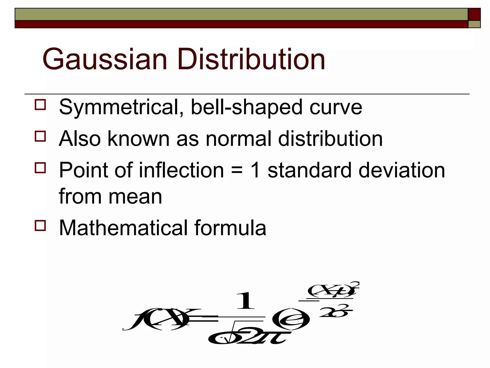
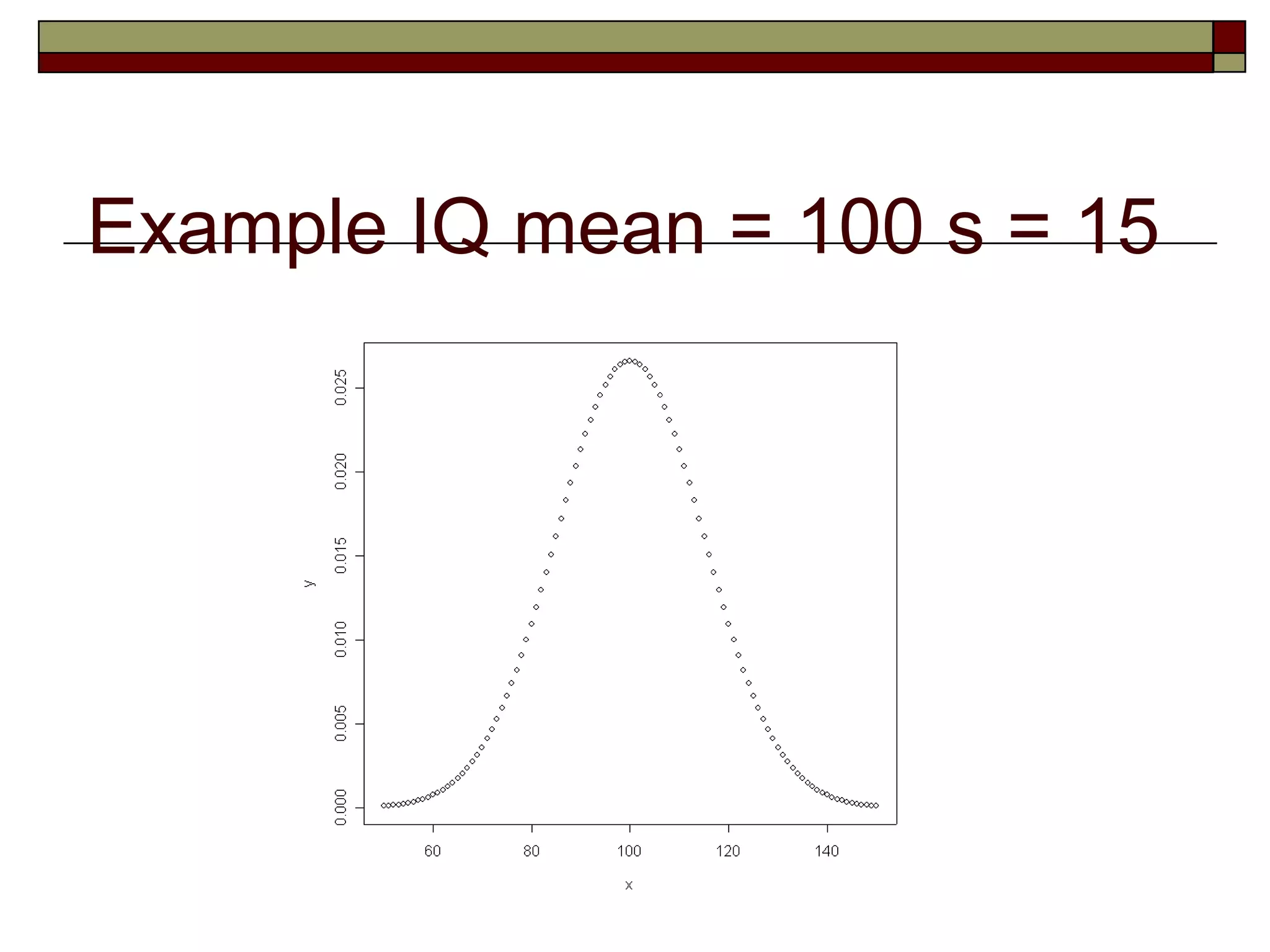
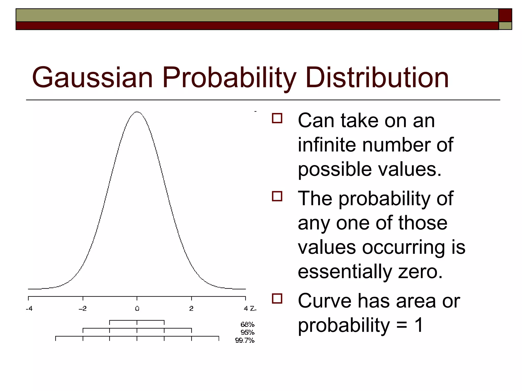
The document introduces the Gaussian or normal distribution, its key properties, and how it can be used for inference. The Gaussian distribution is symmetrical and bell-shaped. It is completely defined by its mean and standard deviation. By transforming data into z-scores, the standard normal distribution can be applied to understand the probabilities of outcomes in any normal distribution. The Gaussian distribution and z-scores allow researchers to assess likelihoods and make inferences about variable values based on their known distribution.

1. Gaussian
Distribution
( normal Distribution)
Manzara Arshad
Roll no. 0151-BH-CHEM-11
Government college university, Lahore

2. Objectives
 Introduce the Gaussian Distribution
 Properties of the Standard Gaussian
Distribution
 Introduce the Central Limit Theorem
 Use Gaussian Distribution in an
inferential fashion

3. Theoretical Distribution
 Empirical distributions
 based on data
 Theoretical distribution
 based on mathematics
 derived from model or estimated from data

4. Gaussian Distribution
Why are Gaussian distributions so important?
 Many dependent variables are commonly
assumed to be normally distributed in the
population
 If a variable is approximately normally
distributed we can make inferences about
values of that variable
 Example: Sampling distribution of the mean

5. So what?
 Remember the Binomial distribution
 With a few trials we were able to calculate
possible outcomes and the probabilities of those
outcomes
 Now try it for a continuous distribution with an infinite
number of possible outcomes. Yikes!
 The Gaussian distribution and its properties are well
known, and if our variable of interest is normally
distributed, we can apply what we know about the
Gaussian distribution to our situation, and find the
probabilities associated with particular outcomes

6. Gaussian Distribution
 Symmetrical, bell-shaped curve
 Also known as normal distribution
 Point of inflection = 1 standard deviation
from mean
 Mathematical formula
f(X)=
1
σ2π
(e)
−
(X−µ)2
2σ2

7.  Since we know the shape of the curve, we can
calculate the area under the curve
 The percentage of that area can be used to
determine the probability that a given value
could be pulled from a given distribution
 The area under the curve tells us about the probability-
in other words we can obtain a p-value for our result
(data) by treating it as a normally distributed data
set.

8. Key Areas under the Curve
 For Gaussian
distributions
+ 1 SD ~ 68%
+ 2 SD ~ 95%
+ 3 SD ~ 99.9%

9. Example IQ mean = 100 s = 15

10.  Problem:
 Each Gaussian distribution with its own
values of m and s would need its own
calculation of the area under various points
on the curve

11. Gaussian Probability Distributions
Standard Normal Distribution – N(0,1)
 We agree to use the
standard Gaussian
distribution
 Bell shaped
 µ=0
 σ=1
 Note: not all bell shaped
distributions are normal
distributions

12. Gaussian Probability Distribution
 Can take on an
infinite number of
possible values.
 The probability of
any one of those
values occurring is
essentially zero.
 Curve has area or
probability = 1

13. Gaussian Distribution
 The standard Gaussian distribution will
allow us to make claims about the
probabilities of values related to our own
data
 How do we apply the standard Gaussian
distribution to our data?

14. Z-score
If we know the population mean and
population standard deviation, for any
value of X we can compute a z-score by
subtracting the population mean and
dividing the result by the population
standard deviation
z=
X−µ
σ

15. Important z-score info
 Z-score tells us how far above or below the mean a value is
in terms of standard deviations
 It is a linear transformation of the original scores
 Multiplication (or division) of and/or addition to (or
subtraction from) X by a constant
 Relationship of the observations to each other remains
the same
Z = (X-m)/s
then
X = sZ + m
[equation of the general form Y = mX+c]

16. Probabilities and z scores: z tables
 Total area = 1
 Only have a probability from width
 For an infinite number of z scores each point has a
probability of 0 (for the single point)
 Typically negative values are not reported
 Symmetrical, therefore area below negative value =
Area above its positive value
 Always helps to draw a sketch!

17. Probabilities are depicted by areas under the curve
 Total area under the curve is
1
 The area in red is equal to
p(z > 1)
 The area in blue is equal to
p(-1< z <0)
 Since the properties of the
normal distribution are
known, areas can be looked
up on tables or calculated on
computer.

18. Strategies for finding probabilities for the
standard normal random variable.
 Draw a picture of standard normal
distribution depicting the area of
interest.
 Re-express the area in terms of
shapes like the one on top of the
Standard Normal Table
 Look up the areas using the table.
 Do the necessary addition and
subtraction.

19. Suppose Z has standard normal
Guassian Find p(0<Z<1.23)

20. Find p(-1.57<Z<0)

21. Find p(Z>.78)

22. Z is standard normal
Calculate p(-1.2<Z<.78)

23. Example
 Data come from distribution: m = 10, s =
3
 What proportion fall beyond X=13?
 Z = (13-10)/3 = 1
 =normsdist(1) or table ⇒ 0.1587
 15.9% fall above 13

24. Example: IQ
 A common example is IQ
 IQ scores are theoretically normally
distributed.
 Mean of 100
 Standard deviation of 15

25. IQ’s are normally distributed with mean 100 and standard
deviation 15. Find the probability that a randomly selected
person has an IQ between 100 and 115
(100 115)
(100 100 100 115 100)
100 100 100 115 100
(
15 15 15
(0 1) .3413
P X
P X
X
P
P Z
< < =
− < − < − =
− − −
< < =
< < =

26. Say we have GRE scores are normally distributed with mean 500 and
standard deviation 100. Find the probability that a randomly selected
GRE score is greater than 620.
 We want to know what’s the probability of
getting a score 620 or beyond.
 p(z > 1.2)
 Result: The probability of randomly getting a
score of 620 is ~.12
620 500
1.2
100
z
−
= =

27. Work time...
 What is the area for scores less than z = -1.5?
 What is the area between z =1 and 1.5?
 What z score cuts off the highest 30% of the
distribution?
 What two z scores enclose the middle 50% of the
distribution?
 If 500 scores are normally distributed with mean = 50
and SD = 10, and an investigator throws out the 20
most extreme scores, what are the highest and lowest
scores that are retained?

28. Standard Scores
 Z is not the only transformation of scores to
be used
 First convert whatever score you have to a z
score.
 New score – new s.d.(z) + new mean
 Example- T scores = mean of 50 s.d. 10
 Then T = 10(z) + 50.
 Examples of standard scores: IQ, GRE, SAT

29. Wrap up
 Assuming our data is normally distributed
allows for us to use the properties of the normal
distribution to assess the likelihood of some
outcome
 This gives us a means by which to determine
whether we might think one hypothesis is more
plausible than another (even if we don’t get a
direct likelihood of either hypothesis)