Anova.pptx

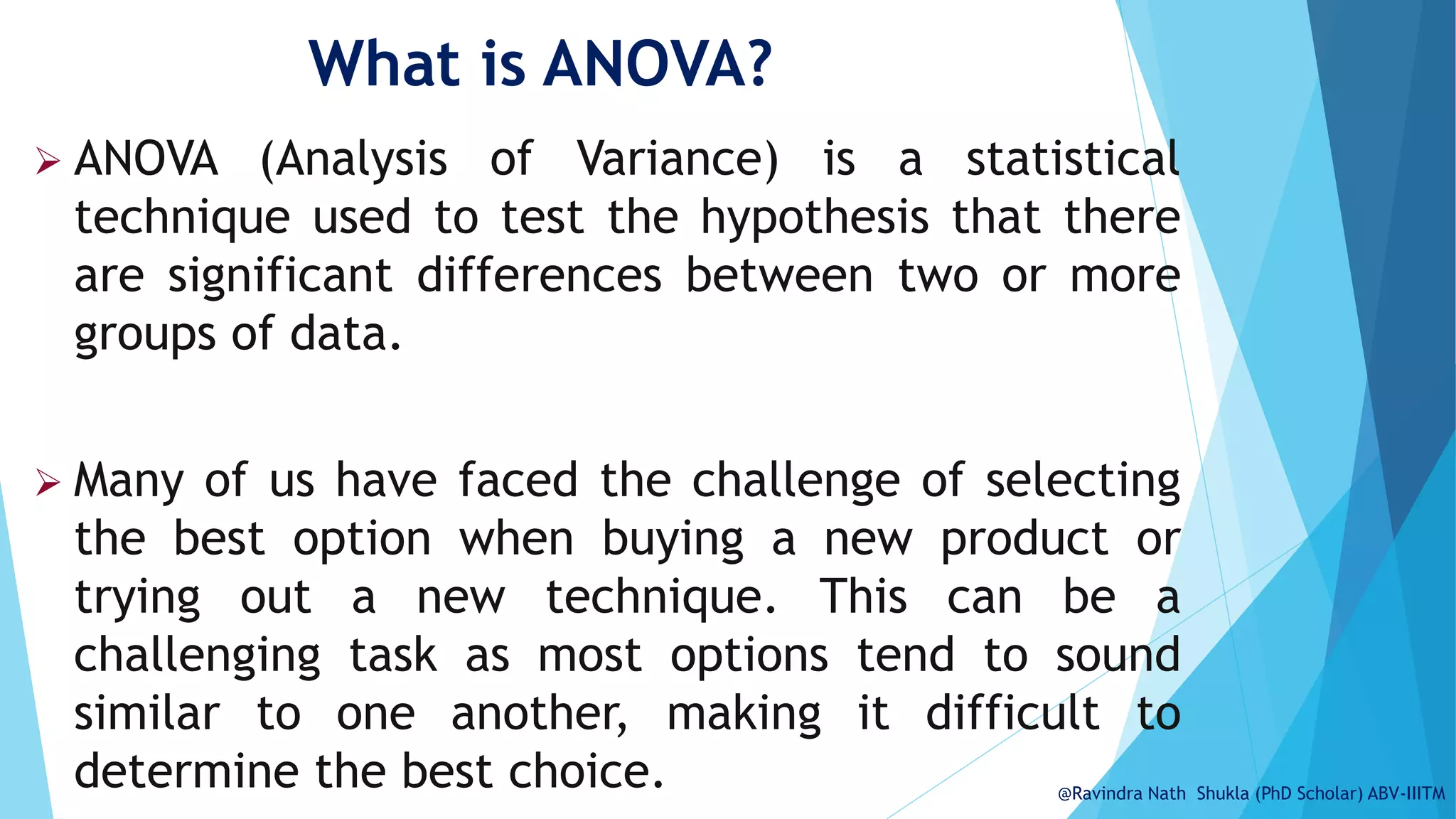
MBMG-7104/ ITHS-2202/ IMAS-3101/ IMHS-3101
@Ravindra Nath Shukla (PhD Scholar) ABV-IIITM

What is ANOVA?
 ANOVA (Analysis of Variance) is a statistical
technique used to test the hypothesis that there
are significant differences between two or more
groups of data.
 Many of us have faced the challenge of selecting
the best option when buying a new product or
trying out a new technique. This can be a
challenging task as most options tend to sound
similar to one another, making it difficult to
determine the best choice. @Ravindra Nath Shukla (PhD Scholar) ABV-IIITM

 In such a situation, to decide the best alternative
we use ANOVA.
 In ANOVA, the goal is to compare the means of
two or more groups and determine whether any
observed differences are statistically significant
or due to chance.
 It compares the variation within groups with the
variation between groups to determine whether
any differences observed are statistically
significant.

How ANOVA Works ?
Consider a scenario where we have three
medical treatments for patients with similar
diseases. Once we have the test results, one
approach is to assume that the treatment
which took the least time to cure the
patients is the best among them. What if
some of these patients had already been
partially cured, or if any other medication
was already working on them?..

 In order to make a confident and reliable decision, we
will need evidence to support our approach. This is
where the concept of ANOVA comes into play.

 A common approach to figuring out a reliable treatment
method would be to analyze the days the patients took to
be cured.
 The statistical technique can be used to compare could be
– Simple t-test, or ANOVA.
 We use “t-test”, When we have only two samples
 In such case, t-test, and ANOVA give the same results.

 However, using a t-test would not be reliable in cases with
more than 2 samples.
 If we conduct multiple t-tests for comparing more than
two samples, it will have a compounded effect on the
error rate of the result.
 For more-than 2 samples, we use ANOVA test.
 ANOVA compares the samples based on their means.

Terminologies Related to ANOVA
 Mean :- There are two kinds of means that we use in
ANOVA calculations, which are separate sample means and
Grand mean.
 Simple or group means
 Overall or Grand Mean(𝜇) =
=(Sum of all data points) / (Total number of data points)
= mean of group means
=
𝑋1+𝑋2+𝑋3……..+𝑋𝑘
𝑛1+𝑛2+𝑛3+ …..𝑛𝑘
𝜇1, 𝜇2, 𝜇3 = 𝑋1, 𝑋2, 𝑋3

 Null Hypothesis :- the null hypothesis states that there
is no significant difference among the means of two or
more groups.
 Specifically, the null hypothesis for ANOVA is that the
population means of all groups are equal.
 Mathematically, the null hypothesis for ANOVA can be
expressed as:
H0: µ1 = µ2 = µ3 = ... = µk
where µ1, µ2, µ3,..., µk are the population means of k
groups being compared in the ANOVA. @Ravindra Nath Shukla (PhD Scholar) ABV-IIITM

 Alternative Hypothesis :- The alternative hypothesis
for ANOVA, which is the opposite of the null hypothesis,
is that at least one of the population means is different
from the others.
 Mathematically, the alternative hypothesis for ANOVA
can be expressed as:
Ha: At least one µi is different from the others,
where i = 1, 2, 3,..., k.

Classification of ANOVA
There are two main types of
ANOVA:
1. One-Way ANOVA: Used to
compare the means of two or
more groups when there is only
one independent variable.
2. Two-Way ANOVA: Used to
compare the means of two or
more groups when there are
two independent variables.

STEPS INVOLVED IN One-way ANOVA test :-
1. Set up the null and alternative hypotheses.
2. Calculate the mean and variance for each group.
3. Calculate the total sum of squares (SST), which
measures the total variation in the data:
SST = Σ(xi - x̄)2
4. Calculate the sum of squares between groups (SSB),
which measures the variation between the group
means:
SSB = nΣ(x̄i - x̄)2

5. Calculate the sum of squares within groups (SSW),
which measures the variation within each group:
SSW = Σ(xi - x̄i)2
6. Calculate the degrees of freedom (df) for each source
of variation:
• Total df = N - 1
• Between df = k - 1
• Within df = N - k
Where’s N= Total no. of observations, and k= No. of groups
7. 7. Calculate the mean square between (MSB) and mean
square within (MSW):
MSB = SSB / dfbetween
MSW = SSW / dfwithin @Ravindra Nath Shukla (PhD Scholar) ABV-IIITM

8. Calculate the F : To calculate the F-statistic, we divide
the mean square between (MSB) by the mean square
within (MSW):
F = MSB / MSW
9. Compare the calculated value of F with the table value
of F (at 5% level of significancy)
10. Decision: Ftable > Fcalculated accept the null hypothesis
If Ftable < Fcalculated reject the null hypothesis

Reading F-distribution table -
The F-distribution table is a table that shows the critical
values of the F distribution. To use the F distribution
table, you only need three values:
The numerator degrees of freedom
The denominator degrees of freedom
The alpha level (common choices are 0.01, 0.05, and
0.10)

Reading F-distribution table -

Illustration 1:
As head of a department of a consumer's research
organization, you have the responsibility for testing and
comparing lifetimes of four brands of electric bulbs.
Suppose you test the lifetime of three electric bulbs of
each of the four brands. The data is shown below, each
entry representing the lifetime of an electric bulb,
measured in hundreds of hours:
A B C D
20 25 24 23
19 23 20 20
21 21 22 20

Solution :
ANOVA TABLE
Source of
Variation
Sum of
Squares SS
Degree
of
freedom
(d.f.)
Mean Square MS Variance
Ratio F
Between
sample
SSB k-1 MSB = SSB/k-1 F = MSB/MSW
Within
Samples
SSW(= SST-
SSB)
n- k MSW = SSW/ n- k
Total SST n- 1

Source of
Variation
Sum of
Squares SS
Degree
of
freedom
(d.f.)
Mean Square MS Variance
Ratio F
Between
sample
SSB = 15 k-1=3 MSB = SSB/k-1 =
15 / 4-1 = 5
F = MSB/MSW
= 5/3 =1.67
Within
Samples
SSW(= SST-
SSB) = 24
n- k= 8 MSW = SSW/ n- k =
24/12-4 = 24/8 =3
Total SST = 39 n- 1 = 11
From F-distribution table Ftable(3,8) = 4.0662.
Since Ftable(3,8), > F calculated Null hypothesis is accepted
ANOVA TABLE

Two-way ANOVA Test
When it is believed that two independent factors might
have an effect on the response variable of interest.
Then ANOVA is used to test for the effects the two factors
simultaneously. Such a test is called two-factor (way)
analysis of variance or Two-way ANOVA.
We test two sets of hypothesis with the same data at the
same time.

Source of
Variation
SS d.f Mean Square MS Variance Ratio F
Between columns SSC c-1 MSC = SSC/(c-1) FClm = Greater Variance / Smaller
variance from MSE & MSC
Between rows SSR r- 1 MSR = SSR/(r-1) Frow = Greater Variance / Smaller
variance from MSE & MSR
Residual SSE (c-1)(r-1) MSE = SSE/ (c-1)(r-1)
Total SST rc - 1
SSC = Sum of squares between columns , SSR = Sum of squares between rows
SSE = Sum of squares for the Error terms (residual) = SST – SSC – SSR
SST = Total sum of squares.
The procedure for analysis of variance is somewhat different from
one-way ANOVA.
In a two-way classification, the analysis of variance table takes the
following form:

Solution :-
Null hypothesis (H0): There is no significant difference
between the sales of salesmen and that of seasons.
The above data are classified according to criteria (i)
salesman and (ii) season.
Overall mean 𝑋 = 360/12 = 30
Salesman Total
Season A B C D
Summer 36 36 21 35 128
Winter 28 29 31 32 120
Mansoon 26 28 29 29 112
TOTAL 90 93 81 96 360

Solution :-
Source of
Variation
SS d.f Mean Square MS Variance Ratio F
Between
columns
SSC = 42 c-1= 3 MSC = SSC/(c-1)
= 14
FClm = MSE / MSC
= 1.619
Between
rows
SSR
= 32
r- 1= 2 MSR = SSR/(r-1)
= 16
Frow = MSE/ MSR
= 1.417
Residual SSE = 136 (c-1)(r-1) = 6 MSE = SSE/(c-1)(r-1)
= 22.67
Total SST = 210 rc - 1= 11
Ftable (3,6) = 4.7571, & Ftable (2,6) = 5.1433
From F-distribution table Ftable > Fcalculated
For both column and row groups, hence Null hypothesis is accepted.

STEPS INVOLVED IN Two-way ANOVA test :-
1. Set up the null and alternative hypotheses.
2. Calculate the mean and variance for column & row
group and Calculate Grand mean.
3. Calculate the total sum of squares (SST), which
measures the total variation in the data:
SST = Σ(xi - x̄)2
4. Calculate the sum of squares between column and row
groups (SSC & SSR), which measures the variation
between the group means:
SSC = nΣ(x̄ic - x̄)2 ; SSR = nΣ(x̄ir - x̄)2

5. Calculate the Sum of squares for the Error terms (residual)
(SSE) :
SSE = SST- SSC-SSR
6. Calculate the degrees of freedom (df) for each source of
variation:
• DF(b/wC) = c - 1 = 4 - 1 = 3
• DF(b/wR) = r – 1 = 3-1 = 2
• DF(residual) = (c-1)(r-1) = 2 x 3 = 6
• DF(total) = rc – 1 = 12-1=11
Where’s c = no. of columns, r= no. of rows
7. Calculate the mean square for columns, row, and residuals :
MSC(b/wC) = SSC / DF(b/wC)
MSR(b/wR) = SSR / DF(b/wR)
MSE(residual) = SSE/ (c-1)(r-1) @Ravindra Nath Shukla (PhD Scholar) ABV-IIITM

8. Calculate the F-statistic for column and row factor:
•Fclm(a,c) = Greater Variance / Smaller variance from MSE & MSC
•Frow(b,c) = Greater Variance / Smaller variance from MSE & MSR
9. Compare the calculated value of F with the table value of
F (at 5% level of significancy)
10. Decision: Ftable > Fcalculated accept the null hypothesis
If Ftable < Fcalculated reject the null hypothesis

Exercise:
Q1. The Amit Merchandising Company wishes to test whether its three
salesmen A, B and C tend to make sales of the same size or whether
they differ in their selling ability as measured by the average size of
their sales. During the last week out of 14 sales, A made 5, B made 4
and C made 5 calls. The following are the weekly sales (in Rs.
Thousand) record of the salesmen:
Test, whether the three salesmen's average sales differ in size.

Exercise:
Q2. Four machines A, B, C and D are used to produce a certain kind of cotton
fabrics. Samples of size 4 with each unit as 100 square meters are
selected from the outputs of the machines at random, and the number
of flaws in each 100 square meters are counted, with the following
result.
Do you think that there is a significant difference in the performance of
the four machines?

Exercise:
Q3. The following data represent the number of units of production per day
turned out by 5 different workers using 4 different types of machines:
Test (a) Whether the mean productivity is the same for 4 different machine
types.
(b) Whether the 5 workers differ with respect to mean productivity.

Anova.pptx

More Related Content

What's hot

Similar to Anova.pptx

More from Ravindra Nath Shukla

Recently uploaded

Anova.pptx