Downloaded 10 times


![Binomial Distribution Solution*
n = 12, p = .20
A. p(0) = .0687
B. p(2) = .2835
C. p(at most 2) = p(0) + p(1) + p(2)
= .0687 + .2062 + .2835
= .5584
D. p(at least 2) = p(2) + p(3)...+ p(12)
= 1 – [p(0) + p(1)]
= 1 – .0687 – .2062
= .7251
@Ravindra Nath Shukla (PhD Scholar) ABV-IIITM](https://image.slidesharecdn.com/discretedistribution-230412040831-e480a821/75/Discrete-Distribution-pptx-39-2048.jpg)


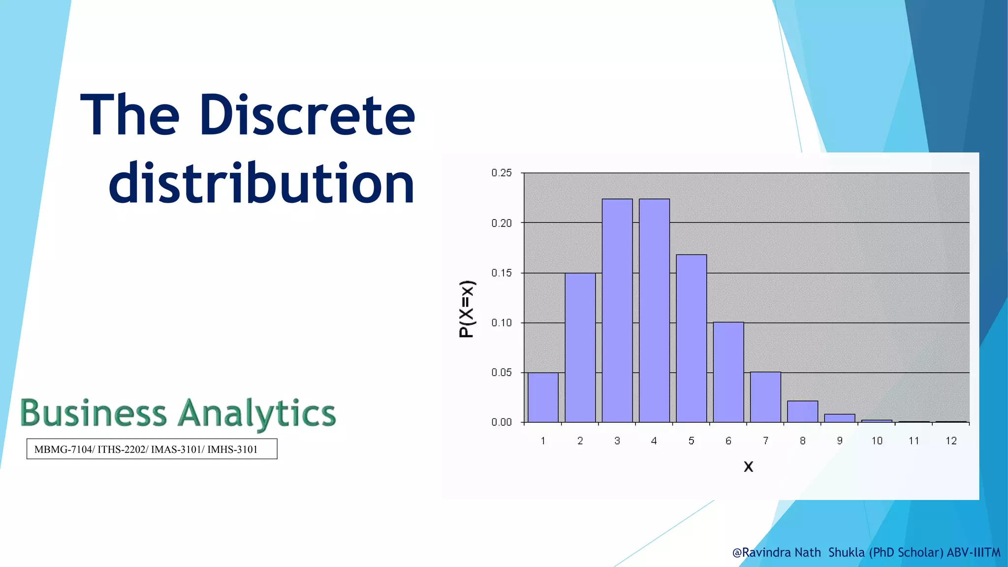
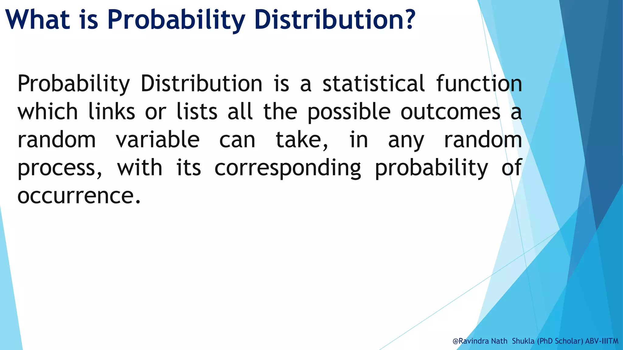
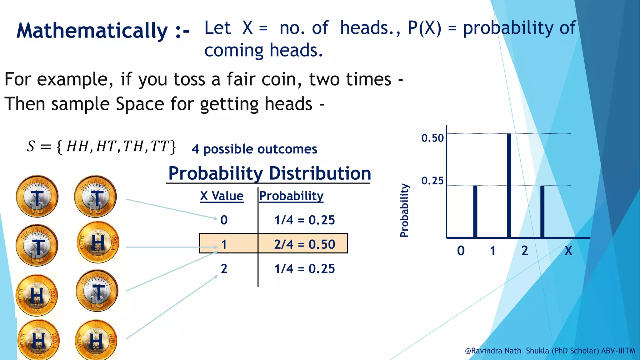
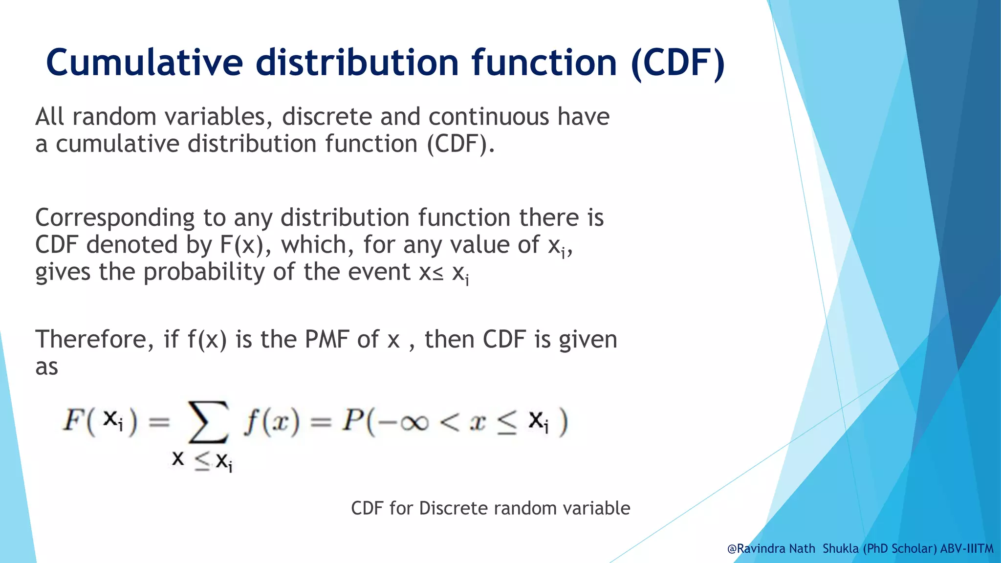
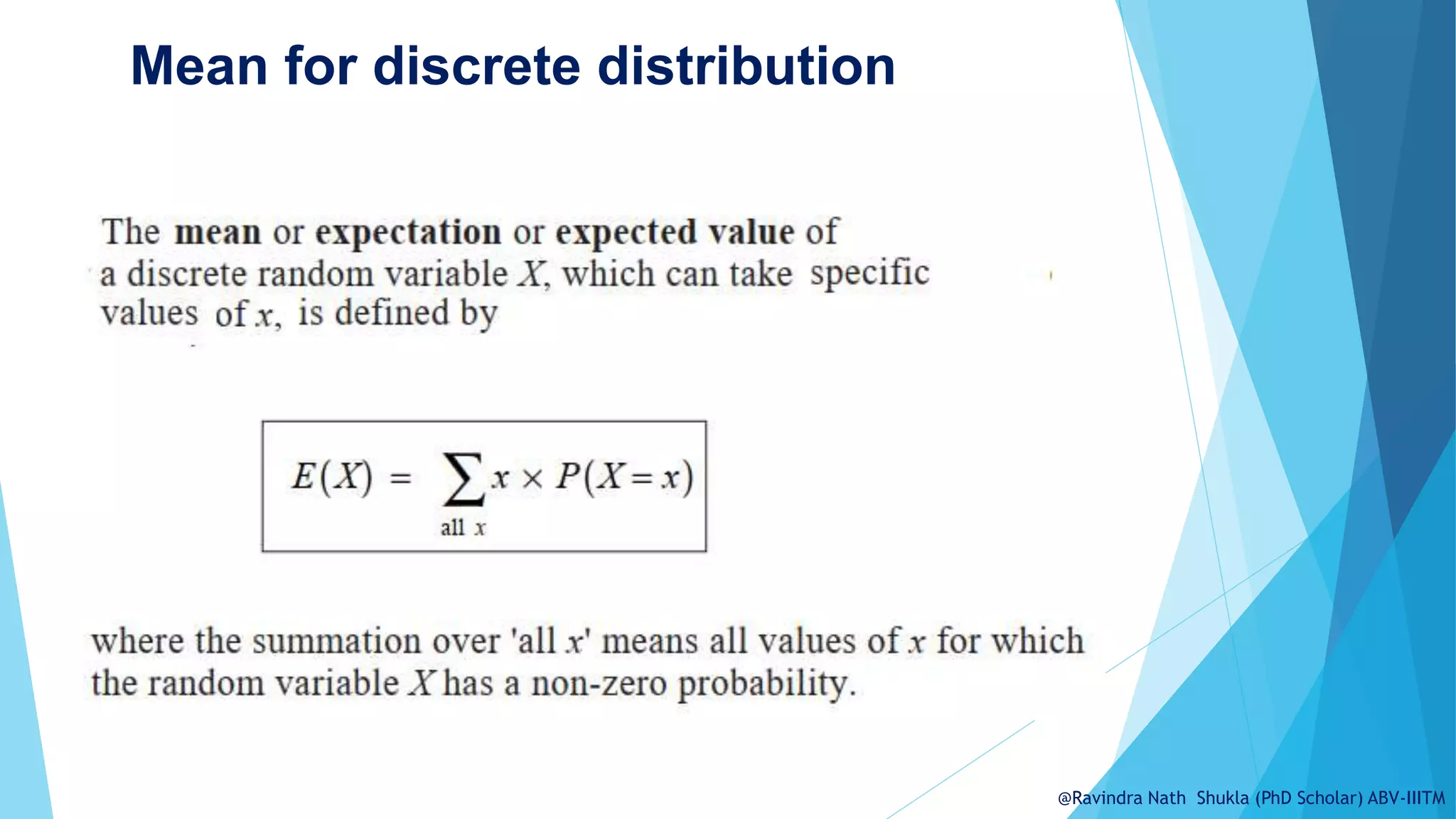
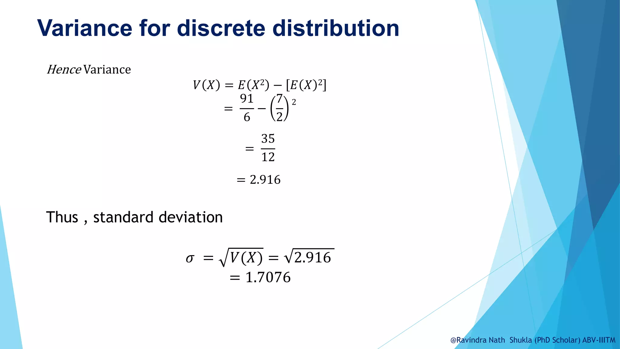
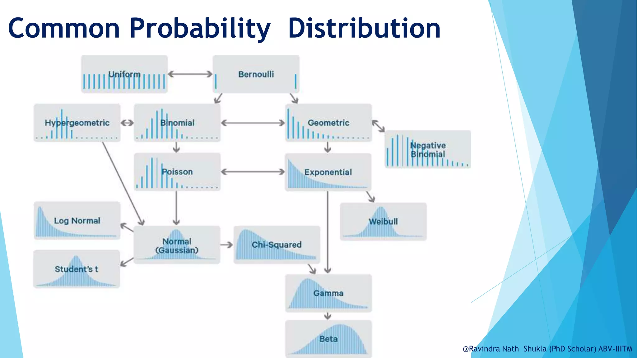
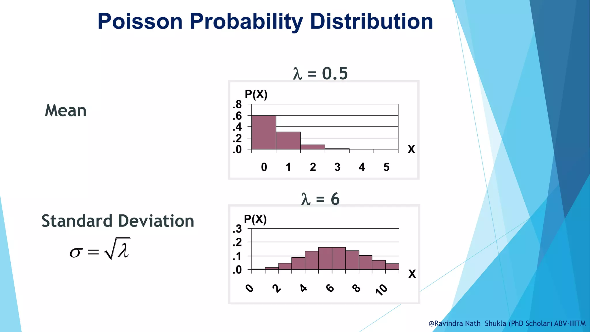
The document discusses probability distributions, specifically discrete distributions, and explains their mathematical foundation, including probability mass functions (pmf) and cumulative distribution functions (cdf). Examples, such as tossing a coin or rolling a die, illustrate concepts like expected value, variance, and standard deviation. Additionally, common types of discrete distributions, including binomial and Poisson distributions, are introduced along with practical applications.