Downloaded 256 times


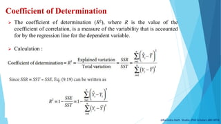


![Calculation b0, b1, and b2
The formula to calculate b1 is:
The formula to calculate b2 is:
The formula to calculate b0 is:
𝑏1
=
[( 𝑋2
2
)( 𝑋1 𝑌) − ( 𝑋1 𝑋2 )( 𝑋2𝑌)]
[( 𝑋1
2
) ( 𝑋2
2
) − ( 𝑋1𝑋2)2]
𝑏2
=
[( 𝑋1
2
) 𝑋2 𝑌) − ( 𝑋1 𝑋2 )( 𝑋1𝑌)]
[( 𝑋1
2
) ( 𝑋2
2
) − ( 𝑋1𝑋2)2]
𝑏0 = 𝑌 − 𝑏1𝑋1 − 𝑏2𝑋2](https://image.slidesharecdn.com/regressionanalysis-240428091142-e351e551/85/Regression-analysis-Simple-Linear-Regression-Multiple-Linear-Regression-45-320.jpg)
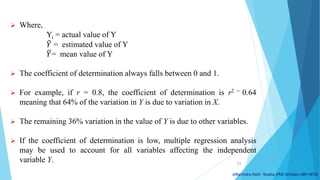
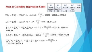
![Step 3: Calculate b0, b1, and b2
Calculation of b1 is:
The formula to calculate b2 is:
The formula to calculate b0 is:
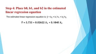
𝑏0 = 𝑌 − 𝑏1𝑋1 − 𝑏2𝑋2 = 6.39 – (0.02622 × 79.6) – (0.1840 × 3.1)
= 6.39 − 2.087− 0.57 =3.733
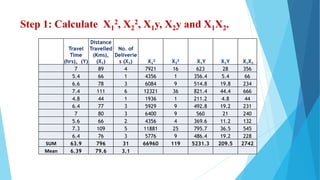
X1
2 X2
2 X1Y X2Y X1X2
Regression
SUM 3598.4 22.9 144.86 11.41 274.4
Mean Y
=6.39
Mean X1=
79.6
Mean X2=
3.1
𝒃𝟏 =
[( 𝑋2
2
)( 𝑋1 𝑌) − ( 𝑋1 𝑋2 )( 𝑋2𝑌)]
[( 𝑋1
2
) ( 𝑋2
2
) − ( 𝑋1𝑋2)2]
=
[ 22.9 × 144.86 − 274.4 × 11.41 ]
[ 3598.4 × 22.9 − (274.4)2]
=
3317.29−3130.90
82403.36−75295.6
=
186.39
7107.76
= 𝟎. 𝟎𝟐𝟔𝟐𝟐
𝒃𝟐 =
[( 𝑋1
2
)( 𝑋2 𝑌) − ( 𝑋1 𝑋2 )( 𝑋1𝑌)]
[( 𝑋1
2
) ( 𝑋2
2
) − ( 𝑋1𝑋2)2]
=
[ 3598.4 × 11.41 − 274.4 × 144.86 ]
[ 3598.4 × 22.9 − (274.4)2]
=
41057.74 − 39749.58
7107.76
=
1308.16
7107.76
= 𝟎. 𝟏𝟖𝟒𝟎](https://image.slidesharecdn.com/regressionanalysis-240428091142-e351e551/85/Regression-analysis-Simple-Linear-Regression-Multiple-Linear-Regression-46-320.jpg)
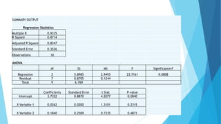
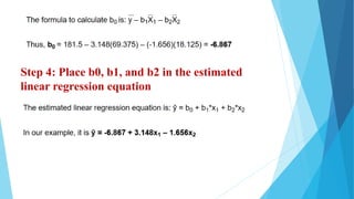


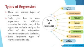
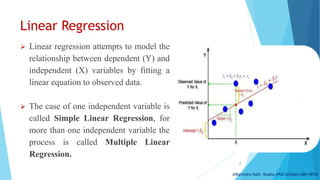
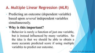
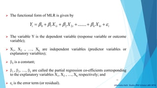
The document discusses regression analysis, which is a statistical process for estimating relationships between dependent and independent variables, often for forecasting purposes. It explains various types of regression, particularly linear regression, and highlights classical assumptions, objectives, and the mathematical framework including the ordinary least squares (OLS) method. Additionally, it covers coefficients of determination and provides an example of demand forecasting based on given data.