Downloaded 15 times

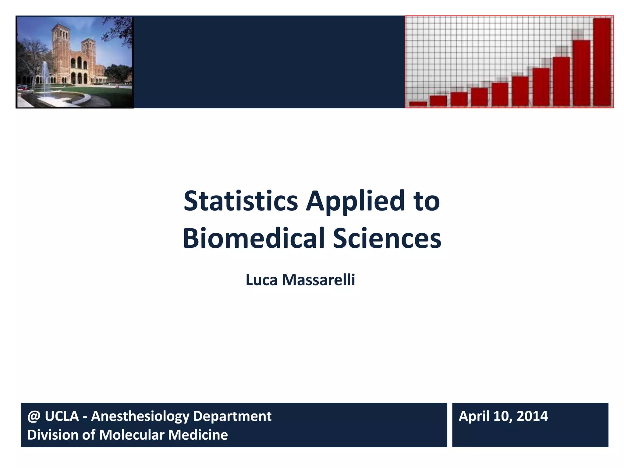

![Estimator has some desirable properties:
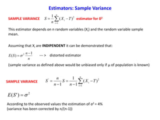
UNBIASED
The estimator is an unbiased estimator of θ if and only if
E(T) = θ --- > (E(T) – θ) = 0
In other words the distance between the average of the collection of estimates and
the single parameter being estimated is null.
Bias is a property of the estimator, not of the estimate.
1}|{|lim
TP
n
EFFICIENCY
The estimator has minimal mean squared error (MSE) or variance of the estimator
MSE(T) = E[T- θ]2
If I have an estimator with smaller dispersion, I will have more probability to find an
estimation which is closer to the TRUE Parameter.
CONSISTENCY
Increasing the sample size increases the probability of the estimator being close to
the population parameter.
Estimators: Properties](https://image.slidesharecdn.com/ucla-statisticpresentation-140609201402-phpapp02/85/Statistics-Applied-to-Biomedical-Sciences-11-320.jpg)
![)(TE
n
TVAR
2
)(
n
StdError
n
i
iX
n
T
1
1
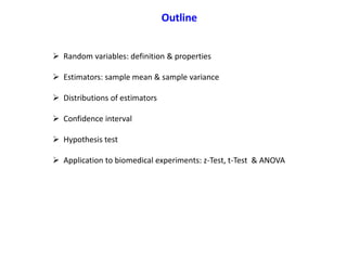
If ),( 2
NX ),(
2
n
NT
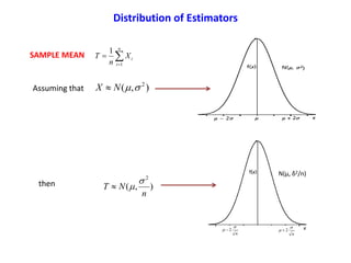
Define an interval around our estimate of μ with confidence coeff. = 95%
1][Pr bTaob
With the transformation to a Standard Normal Distribution
1][Pr
222
n
b
n
T
n
a
ob
1][Pr
22
n
b
Z
n
a
ob
1][Pr
2
12
ZZZob
Confidence Interval of the Mean
Normal Probability Density Function
ProbabilityDensity
x](https://image.slidesharecdn.com/ucla-statisticpresentation-140609201402-phpapp02/85/Statistics-Applied-to-Biomedical-Sciences-21-320.jpg)
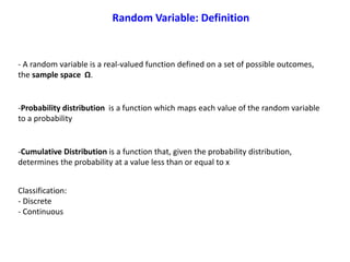
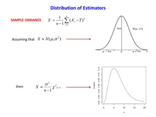
![Here we are assuming σ2 is known. What if the variance is unknown?
1][Pr
2
12
ZZZob
n
Zb
2
2
1
1][Pr bTaob
Zα/2 0 Z1-α/2 a μ b
n
Za
2
2
n
ZCI
2
2
1
Confidence Interval of the Mean](https://image.slidesharecdn.com/ucla-statisticpresentation-140609201402-phpapp02/85/Statistics-Applied-to-Biomedical-Sciences-22-320.jpg)
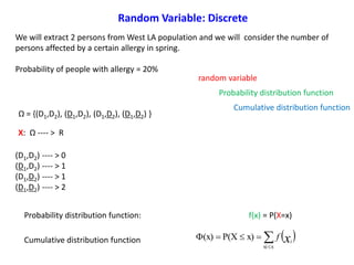
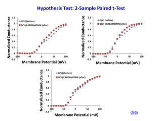
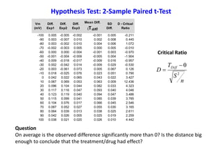
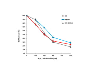
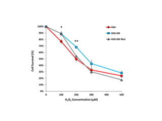
![Question
Based on Mean comparison, on average, did TRTM treatment really change the level
of survival of the general population?
HEK cells
[H2O2] = 200 μM
We assume that the survival probability of HEK cells follows the normal distribution
with the following known parameters.
μ0 = 62%
σ = 15.5%
Assume that one sample of HEK population is extracted and submitted to a certain
treatment (TRTM)
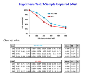
Observed value:
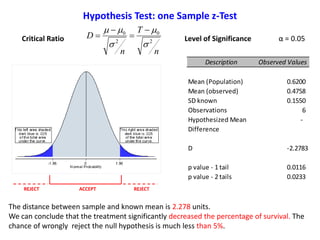
Hypothesis Test: one Sample z-Test
Exp. Observed Values
1 0.605
2 0.592
3 0.661
4 0.367
5 0.323
6 0.307
Sample Mean 0.476
SD 0.160
SE 0.065](https://image.slidesharecdn.com/ucla-statisticpresentation-140609201402-phpapp02/85/Statistics-Applied-to-Biomedical-Sciences-29-320.jpg)
![Question
Based on Mean comparison, on average, did TRTM treatment really change the level
of survival of the general population?
Let’s assume that the survival probability of HEK cells follow the normal distribution
with the following known parameters.
μ0 = 62%
σ = unknown
Assume that one sample of HEK population is extracted and submitted to treatment
TRTM
Observed value:
HEK cells
[H2O2] = 200 μM
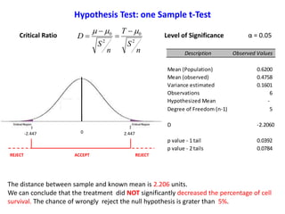
Hypothesis Test: one Sample t-Test
Exp. Observed Values
1 0.605
2 0.592
3 0.661
4 0.367
5 0.323
6 0.307
Sample Mean 0.476
SD 0.160
SE 0.065](https://image.slidesharecdn.com/ucla-statisticpresentation-140609201402-phpapp02/85/Statistics-Applied-to-Biomedical-Sciences-32-320.jpg)
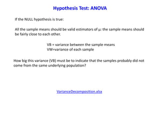
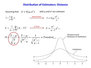
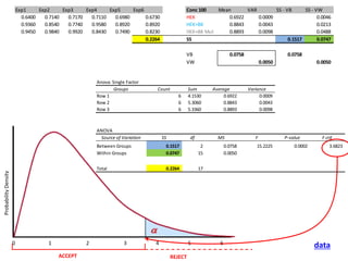
![The variance of the underlying population σ2 could be estimated by 2 different methods:
a) The variance of the sample means
b) The average of the sample variances
1
])(...)()([ 22
22
2
11
K
XxnXxnXxn
VB kk
Assuming that each group has the same n, VB can be simplified as follows:
1
)(
1
2
K
Xxn
VB
K
k
k
K
k
n
i
kik
K
k
k
n
Xx
K
S
K
VW
1 1
2
1
2
1
)(11
Variance Between:
We know that the variance of the sample means is equal to the SE or δ2 /n
Variance Within:
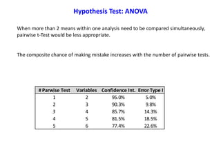
Hypothesis Test: ANOVA](https://image.slidesharecdn.com/ucla-statisticpresentation-140609201402-phpapp02/85/Statistics-Applied-to-Biomedical-Sciences-45-320.jpg)

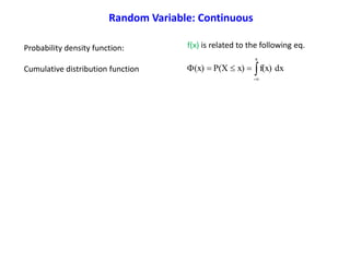
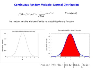
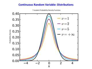
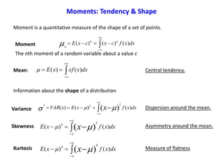
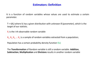
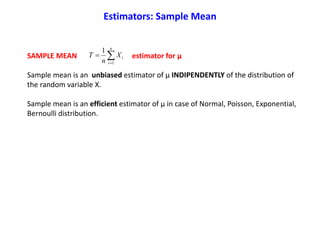
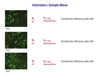
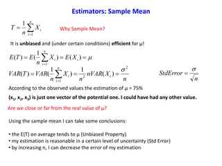
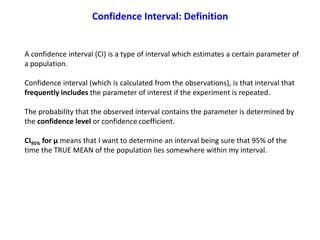
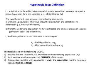
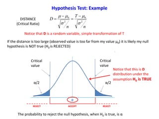
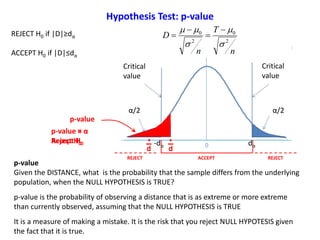
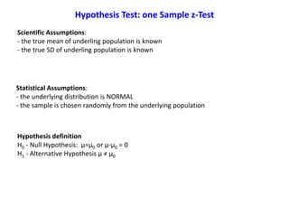
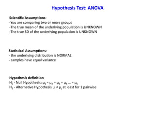
The document provides an overview of key statistical concepts including: - Random variables and their probability distributions and functions - Common estimators like the sample mean and variance - The distributions of common estimators and how they relate to the underlying population parameters - Confidence intervals and how they are used to quantify the uncertainty in estimates based on sample data - Hypothesis testing framework including defining the null and alternative hypotheses, calculating a test statistic, and determining whether to reject or fail to reject the null based on probability thresholds


