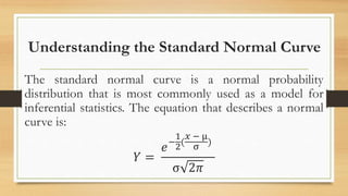
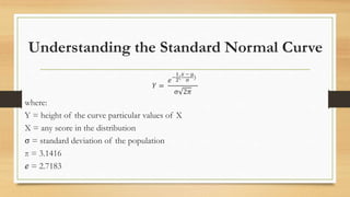
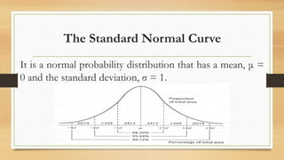
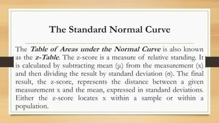
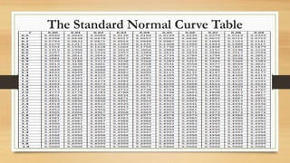
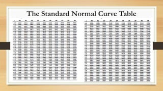
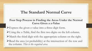
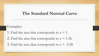
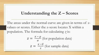
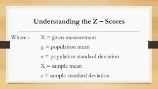
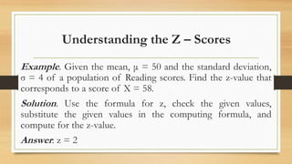
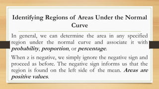
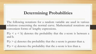
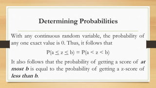
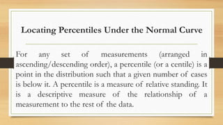
Chapter 3
Understanding Normal
Distribution
Mr. Anthony F. Balatar Jr.
Subject Instructor
Visualizing a Normal Distribution
If a distribution consists of a very large number of cases
and the three measures of averages (mean, median, and
mode) are equal, then the distribution is symmetrical and
the skewness is 0. In Statistics, such distribution is called
normal distribution or simply normal curve.
Visualizing a Normal Distribution
The normal curve has a very important role in inferential
statistics. It provides a graphical representation of
statistical values that are needed in describing the
characteristics of populations as well as in making
decisions. It is defined by an equation that uses the
population mean, μ and the standard deviation, σ.
Properties of the Normal Distribution
The distribution curve is bell-shaped.
The curve is symmetrical about its center.
The mean, the median, and the mode coincide at the
center.
The width of the curve is determined by the standard
deviation of the distribution.
Properties of the Normal Distribution
The tails of the curve flatten out indefinitely along the
horizontal axis, always approaching the axis but never
touching it. That is, the curve is asymptotic to the base
line.
The area under the curve is 1. Thus, it represents the
probability or proportion or the percentage associated
with specific sets of measurement values.
Understanding the Standard Normal Curve
The standard normal curve is a normal probability
distribution that is most commonly used as a model for
inferential statistics. The equation that describes a normal
curve is:
𝑌 =
𝑒−
1
2
(
𝑥 − μ
σ
)
σ 2𝜋
Understanding the Standard Normal Curve
𝑌 =
𝑒−
1
2(
𝑥 − μ
σ )
σ 2𝜋
where:
Y = height of the curve particular values of X
X = any score in the distribution
σ = standard deviation of the population
π = 3.1416
ℯ = 2.7183
The Standard Normal Curve
It is a normal probability distribution that has a mean, μ =
0 and the standard deviation, σ = 1.
The Standard Normal Curve
The Table of Areas under the Normal Curve is also known
as the z-Table. The z-score is a measure of relative standing. It
is calculated by subtracting mean (μ) from the measurement (x)
and then dividing the result by standard deviation (σ). The final
result, the z-score, represents the distance between a given
measurement x and the mean, expressed in standard deviations.
Either the z-score locates x within a sample or within a
population.
The Standard Normal Curve Table
Table of Areas under the Normal Curve (z-Table)
The Standard Normal Curve Table
Table of Areas under the Normal Curve (z-Table)
The Standard Normal Curve
Four Step Process in Finding the Areas Under the Normal
Curve Given a z-Value
Express the given z-value into a three-digit form.
Using the z-Table, find the first two digits on the left column.
Match the third digit with the appropriate column on the right.
Read the area (or probability) at the intersection of the row and
the column. This is the required area.
The Standard Normal Curve
Examples:
1. Find the area that corresponds to z = 1.
2. Find the area that corresponds to z = 1.36.
3. Find the area that corresponds to z = -2.58
Understanding the Z – Scores
The areas under the normal curve are given in terms of z-
values or scores. Either the z-score locates X within a
population. The formula for calculating z is:
𝑧 =
𝑥 − 𝜇
𝜎
(for population data)
𝑧 =
𝑥 −𝑥
𝑠
(for sample data)
Understanding the Z – Scores
Where : X = given measurement
μ = population mean
σ = population standard deviation
X = sample mean
s = sample standard deviation
Understanding the Z – Scores
Example. Given the mean, μ = 50 and the standard deviation,
σ = 4 of a population of Reading scores. Find the z-value that
corresponds to a score of X = 58.
Solution. Use the formula for z, check the given values,
substitute the given values in the computing formula, and
compute for the z-value.
Answer: z = 2
Identifying Regions of Areas Under the Normal
Curve
In general, we can determine the area in any specified
region under the normal curve and associate it with
probability, proportion, or percentage.
When z is negative, we simply ignore the negative sign and
proceed as before. The negative sign informs us that the
region is found on the left side of the mean. Areas are
positive values.
Determining Probabilities
The following notations for a random variable are used in various
solutions concerning the normal curve. Mathematical notations are
convenient forms of lengthy expressions.
P(a < z < b) denotes the probability that the z-score is between a
and b.
P(z > a) denotes the probability that the z-score is greater than a.
P(z < a) denotes the probability that the z-score is less than a.
Determining Probabilities
With any continuous random variable, the probability of
any one exact value is 0. Thus, it follows that
P(a < z < b) = P(a < z < b)
It also follows that the probability of getting a score of at
most b is equal to the probability of getting a z-score of
less than b.
Determining Probabilities
It is important to correctly interpret key phrases such as at
most, at least, more than, no more than, and so on.
Locating Percentiles Under the Normal Curve
For any set of measurements (arranged in
ascending/descending order), a percentile (or a centile) is a
point in the distribution such that a given number of cases
is below it. A percentile is a measure of relative standing. It
is a descriptive measure of the relationship of a
measurement to the rest of the data.
Locating Percentiles Under the Normal Curve
There are three important things to remember when we are
given probabilities and we want to know their corresponding z-
scores:
A probability value corresponds to an area under the normal
curve.
In the table of Areas Under the Normal Curve, the numbers
in the extreme left and across the top are z-score, which are
the distances along the horizontal scale.

Chapter 2 understanding the normal curve distribution

  • 1.
    Chapter 3 Understanding Normal Distribution Mr.Anthony F. Balatar Jr. Subject Instructor
  • 2.
    Visualizing a NormalDistribution If a distribution consists of a very large number of cases and the three measures of averages (mean, median, and mode) are equal, then the distribution is symmetrical and the skewness is 0. In Statistics, such distribution is called normal distribution or simply normal curve.
  • 3.
    Visualizing a NormalDistribution The normal curve has a very important role in inferential statistics. It provides a graphical representation of statistical values that are needed in describing the characteristics of populations as well as in making decisions. It is defined by an equation that uses the population mean, μ and the standard deviation, σ.
  • 4.
    Properties of theNormal Distribution The distribution curve is bell-shaped. The curve is symmetrical about its center. The mean, the median, and the mode coincide at the center. The width of the curve is determined by the standard deviation of the distribution.
  • 5.
    Properties of theNormal Distribution The tails of the curve flatten out indefinitely along the horizontal axis, always approaching the axis but never touching it. That is, the curve is asymptotic to the base line. The area under the curve is 1. Thus, it represents the probability or proportion or the percentage associated with specific sets of measurement values.
  • 6.
    Understanding the StandardNormal Curve The standard normal curve is a normal probability distribution that is most commonly used as a model for inferential statistics. The equation that describes a normal curve is: 𝑌 = 𝑒− 1 2 ( 𝑥 − μ σ ) σ 2𝜋
  • 7.
    Understanding the StandardNormal Curve 𝑌 = 𝑒− 1 2( 𝑥 − μ σ ) σ 2𝜋 where: Y = height of the curve particular values of X X = any score in the distribution σ = standard deviation of the population π = 3.1416 ℯ = 2.7183
  • 8.
    The Standard NormalCurve It is a normal probability distribution that has a mean, μ = 0 and the standard deviation, σ = 1.
  • 9.
    The Standard NormalCurve The Table of Areas under the Normal Curve is also known as the z-Table. The z-score is a measure of relative standing. It is calculated by subtracting mean (μ) from the measurement (x) and then dividing the result by standard deviation (σ). The final result, the z-score, represents the distance between a given measurement x and the mean, expressed in standard deviations. Either the z-score locates x within a sample or within a population.
  • 10.
    The Standard NormalCurve Table Table of Areas under the Normal Curve (z-Table)
  • 11.
    The Standard NormalCurve Table Table of Areas under the Normal Curve (z-Table)
  • 12.
    The Standard NormalCurve Four Step Process in Finding the Areas Under the Normal Curve Given a z-Value Express the given z-value into a three-digit form. Using the z-Table, find the first two digits on the left column. Match the third digit with the appropriate column on the right. Read the area (or probability) at the intersection of the row and the column. This is the required area.
  • 13.
    The Standard NormalCurve Examples: 1. Find the area that corresponds to z = 1. 2. Find the area that corresponds to z = 1.36. 3. Find the area that corresponds to z = -2.58
  • 14.
    Understanding the Z– Scores The areas under the normal curve are given in terms of z- values or scores. Either the z-score locates X within a population. The formula for calculating z is: 𝑧 = 𝑥 − 𝜇 𝜎 (for population data) 𝑧 = 𝑥 −𝑥 𝑠 (for sample data)
  • 15.
    Understanding the Z– Scores Where : X = given measurement μ = population mean σ = population standard deviation X = sample mean s = sample standard deviation
  • 16.
    Understanding the Z– Scores Example. Given the mean, μ = 50 and the standard deviation, σ = 4 of a population of Reading scores. Find the z-value that corresponds to a score of X = 58. Solution. Use the formula for z, check the given values, substitute the given values in the computing formula, and compute for the z-value. Answer: z = 2
  • 17.
    Identifying Regions ofAreas Under the Normal Curve In general, we can determine the area in any specified region under the normal curve and associate it with probability, proportion, or percentage. When z is negative, we simply ignore the negative sign and proceed as before. The negative sign informs us that the region is found on the left side of the mean. Areas are positive values.
  • 18.
    Determining Probabilities The followingnotations for a random variable are used in various solutions concerning the normal curve. Mathematical notations are convenient forms of lengthy expressions. P(a < z < b) denotes the probability that the z-score is between a and b. P(z > a) denotes the probability that the z-score is greater than a. P(z < a) denotes the probability that the z-score is less than a.
  • 19.
    Determining Probabilities With anycontinuous random variable, the probability of any one exact value is 0. Thus, it follows that P(a < z < b) = P(a < z < b) It also follows that the probability of getting a score of at most b is equal to the probability of getting a z-score of less than b.
  • 20.
    Determining Probabilities It isimportant to correctly interpret key phrases such as at most, at least, more than, no more than, and so on.
  • 21.
    Locating Percentiles Underthe Normal Curve For any set of measurements (arranged in ascending/descending order), a percentile (or a centile) is a point in the distribution such that a given number of cases is below it. A percentile is a measure of relative standing. It is a descriptive measure of the relationship of a measurement to the rest of the data.
  • 22.
    Locating Percentiles Underthe Normal Curve There are three important things to remember when we are given probabilities and we want to know their corresponding z- scores: A probability value corresponds to an area under the normal curve. In the table of Areas Under the Normal Curve, the numbers in the extreme left and across the top are z-score, which are the distances along the horizontal scale.