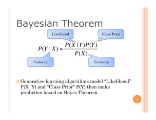
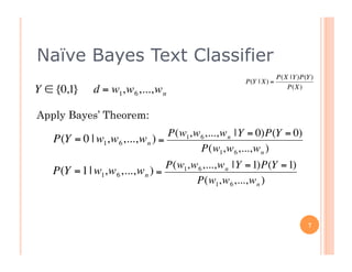
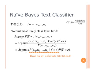
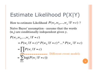
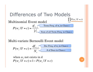
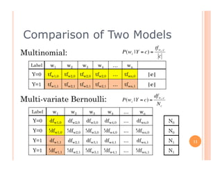
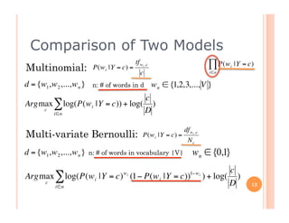
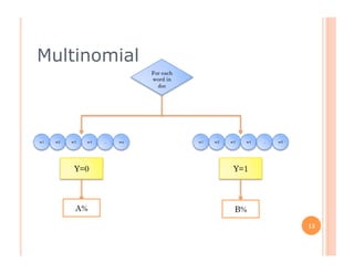
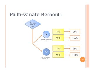
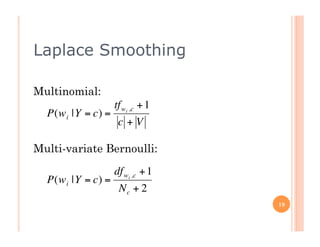
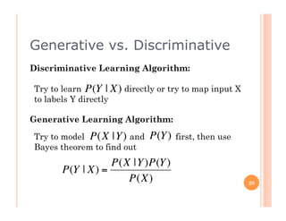
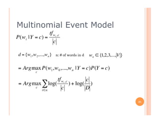
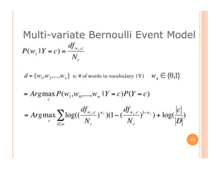
Naive Bayesian Text Classifier Event Models

NAÏVE BAYESIAN
TEXT CLASSIFIER
EVENT MODELS
NOTES AND HOW TO USE THEM
Alex Lin
Senior Architect
Intelligent Mining
alin@intelligentmining.com

Outline
  Quick refresher for
  Naïve Bayesian Text Classifier
  Event Models
  Multinomial Event Model
  Multi-variate Bernoulli Event Model
  Performance characteristics
  Why are they important?

2

Naïve Bayes Text Classifier
  Supervised Learning
  Labeled data set for training to classify the
unlabeled data
  Easy to implement and highly scalable
  It is often the first thing to try

  Successful cases: Email spam filtering,
News article categorization, Product
classification, Social content categorization

3

Bayesian Theorem
Likelihood Class Prior

P(X |Y )P(Y )
P(Y | X) =
P(X)
Posterior Evidence

€  Generative learning algorithms model “Likelihood”
P(X|Y) and “Class Prior” P(Y) then make
prediction based on Bayes Theorem.
6

P(X |Y )P(Y )
P(Y | X) =
P(X)
Y ∈ {0,1} d = w1,w 6 ,...,w n

Apply Bayes’ Theorem: €

P(w1,w 6 ,...,w n |Y = 0)P(Y = 0)
€P(Y = 0 | w1,w 6 ,...,w n ) =
P(w1,w 6 ,...,w n )
P(w1,w 6 ,...,w n |Y = 1)P(Y = 1)
P(Y = 1 | w1,w 6 ,...,w n ) =
P(w1,w 6 ,...,w n )
€
€

€ 7
€

P(X |Y )P(Y )
P(Y | X) =
P(X)
Y ∈ {0,1} d = w1,w 6 ,...,w n

To find most likely class label for d: €
Argmax P(Y = c | w1,w 6 ,...,w n )
€ € c
P(w1,w 6 ,...,w n |Y = c)P(Y = c)
= Argmax
c P(w1,w 6 ,...,w n )
€ = Argmax P(w1,w 6 ,...,w n |Y = c)P(Y = c)
c

How do we estimate likelihood?
€ 8

€

Differences of Two Models
∏ P(w i |Y = c)
Multinomial Event model i∈n

tf wi ,c Term Freq. of wi in Class c
P(w i |Y = c) =
c €
Sum of all Term Freq. in Class c

Multi-variate Bernoulli Event model
€ df wi ,c Doc Freq. of wi in Class c
P(w i |Y = c) = # of Docs in Class c
Nc
when wi not exists in d
10
P(w i |Y = c) = 1− P(w i |Y = c)
€

Comparison of Two Models
tf wi ,c
Multinomial: P(w i |Y = c) =
c
Label w1 w2 w3 w4 … wn
Y=0 tfw1,0 tfw2,0 tfw2,0 tfw2,0 … tfwn,0 |c|
€
Y=1 tfw1,1 tfw2,1 tfw2,1 tfw2,1 … tfwn,1 |c|

df wi ,c
Multi-variate Bernoulli: P(w i |Y = c) =
Nc
Label w1 w2 w3 w4 … wn
Y=0 dfw1,0 dfw2,0 dfw3,0 dfw4,0 … dfwn,0 N0
€
Y=0 !dfw1,0 !dfw2,0 !dfw3,0 !dfw4,0 … !dfwn,0 N0
Y=1 dfw1,1 dfw2,1 dfw3,1 dfw4,1 … dfwn,1 N1 11

Y=1 !dfw1,1 !dfw2,1 !dfw3,1 !dfw4,1 … !dfwn,1 N1

Comparison of Two Models
tf wi ,c ∏ P(w |Y = c)
Multinomial: P(w i |Y = c) =
c i∈n
i

d = {w1,w 2 ,...,w n } n: # of words in d w n ∈ {1,2,3,..., V }
c €
Argmax ∑ log(P(w i |Y = c)) + log( )
€
c
i∈n D
€
df wi ,c
Multi-variate Bernoulli: P(w i |Y = c) =
Nc
d = {w1,w 2 ,...,w n } n: # of words in vocabulary |V| w n ∈ {0,1}
€ c
Argmax ∑ log(P(w i |Y = c) (1− P(w i |Y = c))
wi 1−w i
) + log( )
c
i∈n D 12

€

Multinomial
For each
word in
doc

w1 w2 w3 w4 .. wn w1 w2 w3 w4 .. w5

Y=0 Y=1

A% B%

13

Multi-variate Bernoulli
For each
word in
doc

Y=1 A%
W
Y=0 1-A%
When W does exists
in doc

Y=1 B%
W’
Y=0 1-B%
When W does not
exists in doc
14

Performance Characteristics
  Multinomial would perform better Multi-variate
Bernoulli in most text classification tasks, especially
when vocabulary size |V| >= 1K
  Multinomial perform better when handling data sets
that have large variance in document length
  Multivariate Bernoulli could have the advantage of
dense data set
  Non-text features could be added as additional
Bernoulli variables. However it should not be added to
the vocabulary in Multinomial model
15

Why are they interesting?
  Certaindata points are more suitable for one
event model than the other.
  Example:
  Web page text + “Domain” + “Author”
  Social content text + “Who”
  Product name / desc + “Brand”
  We can create a Naïve Bayes Classifier that
combines event models
  Most importantly, try both on your data set
16

Thank you
  Any question or comment?

17

Appendix
  Laplace Smoothing
  Generative vs Discriminative Learning
  Multinomial Event Model

  Multi-variate Bernoulli Event Model
  Notation

18

Laplace Smoothing

Multinomial:
tf wi ,c + 1
P(w i |Y = c) =
c+V

Multi-variate Bernoulli:

€ df wi ,c + 1
P(w i |Y = c) =
Nc + 2
19

€

Generative vs. Discriminative
Discriminative Learning Algorithm:

Try to learn P(Y | X) directly or try to map input X
to labels Y directly

Generative Learning Algorithm:

Try to model P(X |Y) and
€ P(Y ) first, then use
Bayes theorem to find out
P(X |Y )P(Y )
P(Y | X) =
€ P(X)
€ 20

Multinomial Event Model
tf wi ,c
P(w i |Y = c) =
c

d = {w1,w 2 ,...,w n } n: # of words in d w n ∈ {1,2,3,..., V }

= Argmax P(w1,w 6 ,...,w n |Y = c)P(Y = c)
c
€ €
c tf wi ,c
= Argmax ∑ log( ) + log( )
c
i∈n
c D

21

Multi-variate Bernoulli Event Model
df wi ,c
P(w i |Y = c) =
Nc

d = {w1,w 2 ,...,w n } n: # of words in vocabulary |V| w n ∈ {0,1}

= Argmax P(w1,w 6 ,...,w n |Y = c)P(Y = c)
c
€
df wi ,c
df
€ wi ,c 1−wi c
= Argmax ∑ log(( ) )(1− ( wi
) ) + log( )
c
i∈n
Nc Nc D

22

Notation
  d: a document
  w: a word in a document

  X: observed data attributes

  Y: Class Label

  |V|: number of terms in vocabulary

  |D|: number of docs in training set

  |c|: number of docs in class c

  tf: Term frequency

  df: document frequency

  !df:
23

References
  McCallum, A., Nigam, K.: A comparison of event models for Naive Bayes
text classiﬁcation. In: Learning for Text Categorization: Papers from the AAAI
Workshop, AAAI Press (1998) 41–48 Technical Report WS-98-05
  Metsis, V., Androutsopoulos, I., Paliouras, G.: Spam Filtering with Naive
Bayes – Which Naive Bayes (2006) Third Conference on Email and Anti-Spam
(CEAS)
  Schneider, K: On Word Frequency Information and Negative Evidence in
Naive Bayes Text Classification (2004) España for Natural Language
Processing, EsTAL

24

Naive Bayesian Text Classifier Event Models

Recommended

Recommended

More Related Content

What's hot

What's hot (20)

Viewers also liked

Viewers also liked (20)

Similar to Naive Bayesian Text Classifier Event Models

Similar to Naive Bayesian Text Classifier Event Models (13)

Recently uploaded

Recently uploaded (20)

Naive Bayesian Text Classifier Event Models