Lecture 2: linear SVM in the dual

Lecture 2: Linear SVM in the Dual
Stéphane Canu
stephane.canu@litislab.eu
Sao Paulo 2014
March 12, 2014

Road map
1 Linear SVM
Optimization in 10 slides
Equality constraints
Inequality constraints
Dual formulation of the linear SVM
Solving the dual
Figure from L. Bottou & C.J. Lin, Support vector machine solvers, in Large scale kernel machines, 2007.

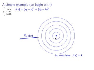
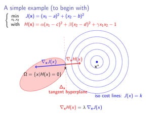
Linear SVM: the problem
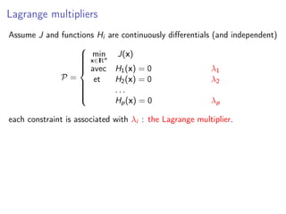
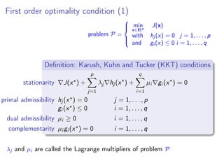
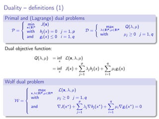
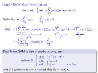
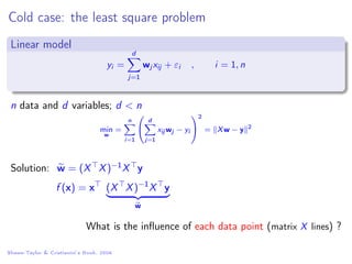
Linear SVM are the solution of the following problem (called primal)
Let {(xi , yi ); i = 1 : n} be a set of labelled data with
xi ∈ IRd
, yi ∈ {1, −1}.
A support vector machine (SVM) is a linear classiﬁer associated with the
following decision function: D(x) = sign w x + b where w ∈ IRd
and
b ∈ IR a given thought the solution of the following problem:
min
w,b
1
2 w 2 = 1
2w w
with yi (w xi + b) ≥ 1 i = 1, n
This is a quadratic program (QP):
min
z
1
2 z Az − d z
with Bz ≤ e
z = (w, b) , d = (0, . . . , 0) , A =
I 0
0 0
, B = −[diag(y)X, y] et e = −(1, . . . , 1)

Road map
1 Linear SVM
Solving the dual

A simple example (to begin with)
min
x1,x2
J(x) = (x1 − a)2 + (x2 − b)2
with
x x
xJ(x)
iso cost lines: J(x) = k

A simple example (to begin with)
min
x1,x2
J(x) = (x1 − a)2 + (x2 − b)2
with H(x) = α(x1 − c)2 + β(x2 − d)2 + γx1x2 − 1
Ω = {x|H(x) = 0}
x x
xJ(x)
∆x
xH(x)
tangent hyperplane
iso cost lines: J(x) = k
xH(x) = λ xJ(x)

The only one equality constraint case
min
x
J(x) J(x + εd) ≈ J(x) + ε xJ(x) d
with H(x) = 0 H(x + εd) ≈ H(x) + ε xH(x) d
Loss J : d is a descent direction if it exists ε0 ∈ IR such that
∀ε ∈ IR, 0 < ε ≤ ε0
J(x + εd) < J(x) ⇒ xJ(x) d < 0
constraint H : d is a feasible descent direction if it exists ε0 ∈ IR such
that ∀ε ∈ IR, 0 < ε ≤ ε0
H(x + εd) = 0 ⇒ xH(x) d = 0
If at x , vectors xJ(x ) and xH(x ) are collinear there is no feasible
descent direction d. Therefore, x is a local solution of the problem.

Lagrange multipliers
Assume J and functions Hi are continuously diﬀerentials (and independent)
P =



min
x∈IRn
J(x)
avec H1(x) = 0
et H2(x) = 0
. . .
Hp(x) = 0

P =



min
x∈IRn
J(x)
avec H1(x) = 0 λ1
et H2(x) = 0 λ2
. . .
Hp(x) = 0 λp
each constraint is associated with λi : the Lagrange multiplier.

P =



min
x∈IRn
J(x)
avec H1(x) = 0 λ1
et H2(x) = 0 λ2
. . .
Hp(x) = 0 λp
each constraint is associated with λi : the Lagrange multiplier.
Theorem (First order optimality conditions)
for x being a local minima of P, it is necessary that:
x J(x ) +
p
i=1
λi x Hi (x ) = 0 and Hi (x ) = 0, i = 1, p

Plan
1 Linear SVM
Solving the dual
Stéphane Canu (INSA Rouen - LITIS) March 12, 2014 8 / 32

The only one inequality constraint case
min
x
J(x) J(x + εd) ≈ J(x) + ε xJ(x) d
with G(x) ≤ 0 G(x + εd) ≈ G(x) + ε xG(x) d
cost J : d is a descent direction if it exists ε0 ∈ IR such that
∀ε ∈ IR, 0 < ε ≤ ε0
J(x + εd) < J(x) ⇒ xJ(x) d < 0
constraint G : d is a feasible descent direction if it exists ε0 ∈ IR such that
∀ε ∈ IR, 0 < ε ≤ ε0
G(x + εd) ≤ 0 ⇒
G(x) < 0 : no limit here on d
G(x) = 0 : xG(x) d ≤ 0
Two possibilities
If x lies at the limit of the feasible domain (G(x ) = 0) and if vectors
xJ(x ) and xG(x ) are collinear and in opposite directions, there is no
feasible descent direction d at that point. Therefore, x is a local solution
of the problem... Or if xJ(x ) = 0

Two possibilities for optimality
xJ(x ) = −µ xG(x ) and µ > 0; G(x ) = 0
or
xJ(x ) = 0 and µ = 0; G(x ) < 0
This alternative is summarized in the so called complementarity condition:
µ G(x ) = 0
µ = 0
G(x ) < 0
G(x ) = 0
µ > 0

First order optimality condition (1)
problem P =



min
x∈IRn
J(x)
with hj (x) = 0 j = 1, . . . , p
and gi (x) ≤ 0 i = 1, . . . , q
Deﬁnition: Karush, Kuhn and Tucker (KKT) conditions
stationarity J(x ) +
p
j=1
λj hj (x ) +
q
i=1
µi gi (x ) = 0
primal admissibility hj (x ) = 0 j = 1, . . . , p
gi (x ) ≤ 0 i = 1, . . . , q
dual admissibility µi ≥ 0 i = 1, . . . , q
complementarity µi gi (x ) = 0 i = 1, . . . , q
λj and µi are called the Lagrange multipliers of problem P

First order optimality condition (2)
Theorem (12.1 Nocedal & Wright pp 321)
If a vector x is a stationary point of problem P
Then there existsa Lagrange multipliers such that x , {λj }j=1:p, {µi }i=1:q
fulfill KKT conditions
a
under some conditions e.g. linear independence constraint qualification
If the problem is convex, then a stationary point is the solution of the
problem
A quadratic program (QP) is convex when. . .
(QP)
min
z
1
2 z Az − d z
with Bz ≤ e
. . . when matrix A is positive definite

KKT condition - Lagrangian (3)
problem P =



min
x∈IRn
J(x)
with hj (x) = 0 j = 1, . . . , p
and gi (x) ≤ 0 i = 1, . . . , q
Deﬁnition: Lagrangian
The lagrangian of problem P is the following function:
L(x, λ, µ) = J(x) +
p
j=1
λj hj (x) +
q
i=1
µi gi (x)
The importance of being a lagrangian
the stationarity condition can be written: L(x , λ, µ) = 0
the lagrangian saddle point max
λ,µ
min
x
L(x, λ, µ)
Primal variables: x and dual variables λ, µ (the Lagrange multipliers)

Duality – deﬁnitions (1)
Primal and (Lagrange) dual problems
P =



min
x∈IRn
J(x)
with hj (x) = 0 j = 1, p
and gi (x) ≤ 0 i = 1, q
D =
max
λ∈IRp,µ∈IRq
Q(λ, µ)
with µj ≥ 0 j = 1, q
Dual objective function:
Q(λ, µ) = inf
x
L(x, λ, µ)
= inf
x
J(x) +
p
j=1
λj hj (x) +
q
i=1
µi gi (x)
Wolf dual problem
W =



max
x,λ∈IRp,µ∈IRq
L(x, λ, µ)
with µj ≥ 0 j = 1, q
and J(x ) +
p
j=1
λj hj (x ) +
q
i=1
µi gi (x ) = 0

Duality – theorems (2)
Theorem (12.12, 12.13 and 12.14 Nocedal & Wright pp 346)
If f , g and h are convex and continuously differentiablea, then the solution
of the dual problem is the same as the solution of the primal
a
under some conditions e.g. linear independence constraint qualification
(λ , µ ) = solution of problem D
x = arg min
x
L(x, λ , µ )
Q(λ , µ ) = arg min
x
L(x, λ , µ ) = L(x , λ , µ )
= J(x ) + λ H(x ) + µ G(x ) = J(x )
and for any feasible point x
Q(λ, µ) ≤ J(x) → 0 ≤ J(x) − Q(λ, µ)
The duality gap is the difference between the primal and dual cost functions

Linear SVM dual formulation - The lagrangian
min
w,b
1
2 w 2
with yi (w xi + b) ≥ 1 i = 1, n
Looking for the lagrangian saddle point max
α
min
w,b
L(w, b, α) with so called
lagrange multipliers αi ≥ 0
L(w, b, α) =
1
2
w 2
−
n
i=1
αi yi (w xi + b) − 1
αi represents the inﬂuence of constraint thus the inﬂuence of the training
example (xi , yi )

Stationarity conditions
L(w, b, α) =
1
2
w 2
−
n
i=1
Computing the gradients:



wL(w, b, α) = w −
n
i=1
αi yi xi
∂L(w, b, α)
∂b
=
n
i=1 αi yi
we have the following optimality conditions



wL(w, b, α) = 0 ⇒ w =
n
i=1
αi yi xi
∂L(w, b, α)
∂b
= 0 ⇒
n
i=1
αi yi = 0

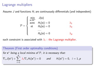
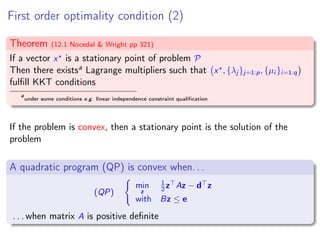
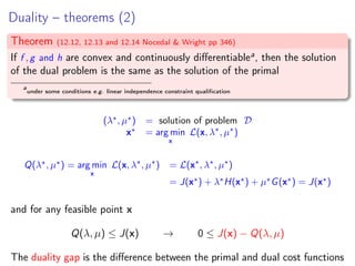
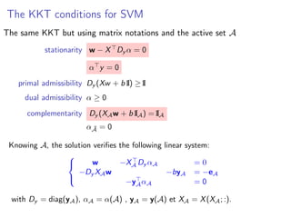
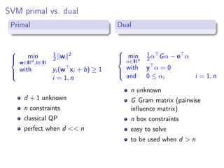
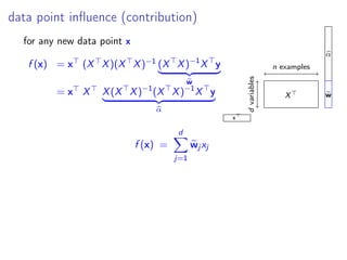
KKT conditions for SVM
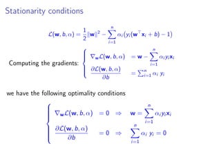
stationarity w −
n
i=1
αi yi xi = 0 and
n
i=1
αi yi = 0
primal admissibility yi (w xi + b) ≥ 1 i = 1, . . . , n
dual admissibility αi ≥ 0 i = 1, . . . , n
complementarity αi yi (w xi + b) − 1 = 0 i = 1, . . . , n
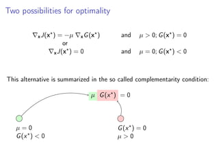
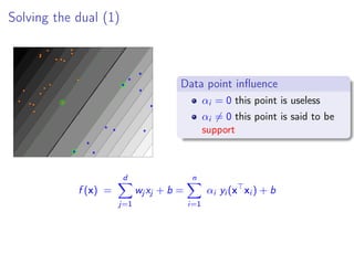
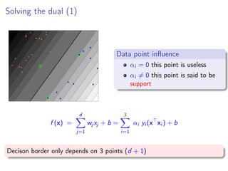
The complementary condition split the data into two sets
A be the set of active constraints: usefull points
A = {i ∈ [1, n] yi (w∗
xi + b∗
) = 1}
its complementary ¯A useless points
if i /∈ A, αi = 0

The KKT conditions for SVM
The same KKT but using matrix notations and the active set A
stationarity w − X Dy α = 0
α y = 0
primal admissibility Dy (Xw + b I1) ≥ I1
dual admissibility α ≥ 0
complementarity Dy (XAw + b I1A) = I1A
α ¯A = 0
Knowing A, the solution veriﬁes the following linear system:



w −XA Dy αA = 0
−Dy XAw −byA = −eA
−yAαA = 0
with Dy = diag(yA), αA = α(A) , yA = y(A) et XA = X(XA; :).

The KKT conditions as a linear system



w −XA Dy αA = 0
−Dy XAw −byA = −eA
−yAαA = 0
with Dy = diag(yA), αA = α(A) , yA = y(A) et XA = X(XA; :).
=
I −XA Dy 0
−Dy XA 0 −yA
0 −yA 0
w
αA
b
0
−eA
0
we can work on it to separate w from (αA, b)

The SVM dual formulation
The SVM Wolfe dual



max
w,b,α
1
2 w 2
−
n
i=1
with αi ≥ 0 i = 1, . . . , n
and w −
n
i=1
αi yi xi = 0 and
n
i=1
αi yi = 0
using the fact: w =
n
i=1
αi yi xi
The SVM Wolfe dual without w and b



max
α
−1
2
n
i=1
n
j=1
αj αi yi yj xj xi +
n
i=1
αi
with αi ≥ 0 i = 1, . . . , n
and
n
i=1
αi yi = 0

Linear SVM dual formulation
L(w, b, α) =
1
2
w 2
−
n
i=1
Optimality: w =
n
i=1
αi yi xi
n
i=1
αi yi = 0
L(α) = 1
2
n
i=1
n
j=1
αj αi yi yj xj xi
w w
−
n
i=1 αi yi
n
j=1
αj yj xj
w
xi − b
n
i=1
αi yi
=0
+
n
i=1 αi
= −
1
2
n
i=1
n
j=1
αj αi yi yj xj xi +
n
i=1
αi
Dual linear SVM is also a quadratic program
problem D



min
α∈IRn
1
2 α Gα − e α
with y α = 0
and 0 ≤ αi i = 1, n
with G a symmetric matrix n × n such that Gij = yi yj xj xi

SVM primal vs. dual
Primal



min
w∈IRd
,b∈IR
1
2 w 2
with yi (w xi + b) ≥ 1
i = 1, n
d + 1 unknown
n constraints
classical QP
perfect when d << n
Dual



min
α∈IRn
1
2α Gα − e α
with y α = 0
and 0 ≤ αi i = 1, n
n unknown
G Gram matrix (pairwise
inﬂuence matrix)
n box constraints
easy to solve
to be used when d > n

SVM primal vs. dual
Primal



min
w∈IRd
,b∈IR
1
2 w 2
with yi (w xi + b) ≥ 1
i = 1, n
d + 1 unknown
n constraints
classical QP
perfect when d << n
Dual



min
α∈IRn
1
2α Gα − e α
with y α = 0
and 0 ≤ αi i = 1, n
n unknown
G Gram matrix (pairwise
inﬂuence matrix)
n box constraints
easy to solve
to be used when d > n
f (x) =
d
j=1
wj xj + b =
n
i=1
αi yi (x xi ) + b

The bi dual (the dual of the dual)


min
α∈IRn
1
2 α Gα − e α
with y α = 0
and 0 ≤ αi i = 1, n
L(α, λ, µ) = 1
2 α Gα − e α + λ y α − µ α
αL(α, λ, µ) = Gα − e + λ y − µ
The bidual 


max
α,λ,µ
−1
2 α Gα
with Gα − e + λ y − µ = 0
and 0 ≤ µ
since w 2
= 1
2 α Gα and DXw = Gα
max
w,λ
−1
2 w 2
with DXw + λ y ≥ e
by identiﬁcation (possibly up to a sign)
b = λ is the Lagrange multiplier of the equality constraint

Cold case: the least square problem
Linear model
yi =
d
j=1
wj xij + εi , i = 1, n
n data and d variables; d < n
min
w
=
n
i=1


d
j=1
xij wj − yi


2
= Xw − y 2
Solution: w = (X X)−1X y
f (x) = x (X X)−1
X y
w
What is the inﬂuence of each data point (matrix X lines) ?
Shawe-Taylor & Cristianini’s Book, 2004

data point inﬂuence (contribution)
for any new data point x
f (x) = x (X X)(X X)−1 (X X)−1
X y
w
= x X X(X X)−1
(X X)−1
X y
α
x
n examples
dvariables
X
α
w
f (x) =
d
j=1
wj xj

data point inﬂuence (contribution)
for any new data point x
f (x) = x (X X)(X X)−1 (X X)−1
X y
w
= x X X(X X)−1
(X X)−1
X y
α
x
n examples
dvariables
X
α
w
x xi
f (x) =
d
j=1
wj xj =
n
i=1
αi (x xi )
from variables to examples
α = X(X X)−1
w
n examples
et w = X α
d variables
what if d ≥ n !

Solving the dual (1)
Data point inﬂuence
αi = 0 this point is useless
αi = 0 this point is said to be
support
f (x) =
d
j=1
wj xj + b =
n
i=1
αi yi (x xi ) + b

Data point inﬂuence
αi = 0 this point is useless
αi = 0 this point is said to be
support
f (x) =
d
j=1
wj xj + b =
3
i=1
αi yi (x xi ) + b
Decison border only depends on 3 points (d + 1)

Assume we know these 3 data points



min
α∈IRn
1
2α Gα − e α
with y α = 0
and 0 ≤ αi i = 1, n
=⇒
min
α∈IR3
1
2α Gα − e α
with y α = 0
L(α, b) =
1
2
α Gα − e α + b y α
solve the following linear system
Gα + b y = e
y α = 0
U = chol(G); % upper
a = U (U’e);
c = U (U’y);
b = (y’*a)(y’*c)
alpha = U (U’(e - b*y));

Conclusion: variables or data point?
seeking for a universal learning algorithm
no model for IP(x, y)
the linear case: data is separable
the non separable case
double objective: minimizing the error together with the regularity of
the solution
multi objective optimisation
dualiy : variable – example
use the primal when d < n (in the liner case) or when matrix G is hard
to compute
otherwise use the dual
universality = nonlinearity
kernels

Lecture 2: linear SVM in the dual

More Related Content

What's hot

Viewers also liked

Similar to Lecture 2: linear SVM in the dual

More from Stéphane Canu

Recently uploaded

Lecture 2: linear SVM in the dual