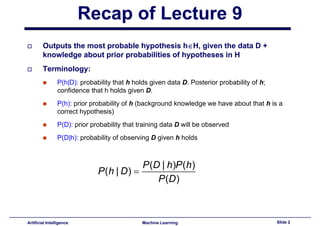
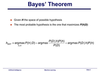
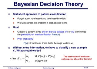
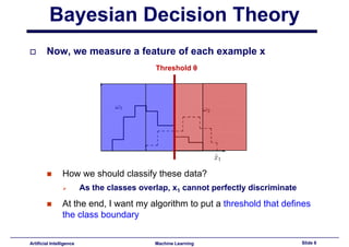
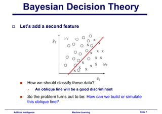
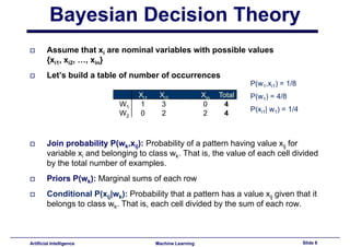
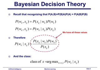
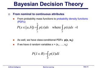
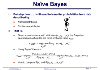
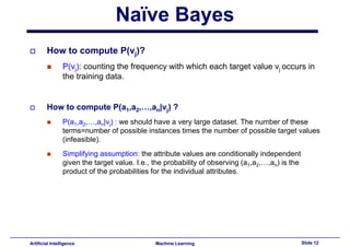
This document provides a summary of Lecture 10 on Bayesian decision theory and Naive Bayes machine learning algorithms. It begins with a recap of Lecture 9 on using probability to classify patterns into categories. It then discusses how to apply these probabilistic concepts to both nominal and continuous variables. A medical example is presented to illustrate Bayesian classification. The document concludes by explaining the Naive Bayes algorithm for classification tasks and providing a worked example of how it is trained and makes predictions.

1. Introduction to Machine
Learning
Lecture 10
Bayesian decision theory – Naïve Bayes
Albert Orriols i Puig
aorriols@salle.url.edu
i l @ ll ld
Artificial Intelligence – Machine Learning
Enginyeria i Arquitectura La Salle
gy q
Universitat Ramon Llull

2. Recap of Lecture 9
Outputs the most probable hypothesis h∈H, given the data D +
knowledge about prior probabilities of hypotheses in H
Terminology:
P(h|D): probability that h holds given data D. Posterior probability of h;
confidence that h holds given D.
P(h): prior probability of h (background knowledge we have about that h is a
correct hypothesis)
P(D): prior probability that training data D will be observed
P(D|h): probability of observing D given h holds
P (D | h )P (h )
P (h | D ) =
P (D )
Slide 2
Artificial Intelligence Machine Learning

3. Bayes’ Theorem
Given H the space of possible hypothesis
The
Th most probable h
b bl hypothesis i the one that maximizes P(h|D)
h i is h h ii P(h|D):
P (D | h )P (h )
hMAP ≡ arg max P (h | D ) = arg max = arg max P (D | h )P (h )
P (D )
h∈H
Slide 3
Artificial Intelligence Machine Learning

4. Today’s Agenda
Bayesian Decision Theory
y y
Nominal Variables
Continuous Variables
A Medical Example
Naïve Bayes
Slide 4
Artificial Intelligence Introduction to C++

5. Bayesian Decision Theory
Statistical approach to pattern classification
pp p
Forget about rule-based and tree-based models
We will express the problem in probabilistic terms
Goal
Classify a pattern x into one of the two classes w1 or w2 to minimize
the probability of misclassification P(error)
Prior
P i probability
b bilit
P(x) = Fraction of times that x belongs to class wk
Without more information, we have to classify a new example
x’. What should we do?
if P ( w1 ) > P ( w2 )
⎧w1 The best option if we know
class of x = ⎨ nothing else about the domain!
⎩w 2 otherwise
Slide 5
Artificial Intelligence Machine Learning

6. Bayesian Decision Theory
Now, we measure a feature of each example x
, p
Threshold θ
How we should classify these data?
As the classes overlap, x1 cannot perfectly discriminate
y
At the end, I want my algorithm to put a threshold that defines
the class boundaryy
Slide 6
Artificial Intelligence Machine Learning

7. Bayesian Decision Theory
Let’s dd
L t’ add a second feature
df t
How we should classify these data?
An oblique line will be a good discriminant
So the problem turns out to be: How can we build or simulate
this oblique line?
Slide 7
Artificial Intelligence Machine Learning

8. Bayesian Decision Theory
Assume that xi are nominal variables with possible values
{xi1, xi2, …, xin}
Let’s build a table of number of occurrences
P(w1,xi1) = 1/8
x
Xi1 Xi2 Xin Total P(w1) = 4/8
4
W1 1 3 0
P(xi1| w1) = 1/4
4
W2 0 2 2
Join probability P(wk,xij): Probability of a pattern having value xij for
variable xi and belonging to class wk. That is, the value of each cell divided
by the total number of examples.
examples
Priors P(wk): Marginal sums of each row
Conditional P(xij| k) P b bilit th t a pattern h a value xij given th t it
C diti l P( |w ): Probability that tt has l i that
belongs to class wk. That is, each cell divided by the sum of each row.
Slide 8
Artificial Intelligence Machine Learning

9. Bayesian Decision Theory
Recall that recognizing that P(A,B)=P(B|A)P(A) = P(A|B)P(B)
g g (,) (|)() (|)()
P ( wk , xij ) = P ( xij | wk ) P ( wk )
P ( wk , xijj ) = P ( wk | xijj ) P ( xijj )
We have all these values
Therefore
P ( xij | wk ) P ( wk )
P ( wk | xij ) =
P ( xij )
And the class:
class of x =arg max k =1, 2 P ( wk | xij )
Slide 9
Artificial Intelligence Machine Learning

10. Bayesian Decision Theory
From nominal to continuous attributes
From probability mass functions to probability density functions
(
(PDFs)
s)
b
P ( x ∈ [a, b]) =∫ p ( x)dx where ∫ p(x)dx =1
a X
As well, we have class-conditional PDFs p(x, wk)
If we have d random variables x = ( 1, …, xd)
e a e a do a ab es (x ,
r rr
P( x ∈ R ) =∫ p ( x )dx
R
Slide 10
Artificial Intelligence Machine Learning

11. Naïve Bayes
But step down… I still need to learn the probabilities from data
p p
described by
Nominal attributes
Continuous attributes
That is,
is
Given a new instance with attributes (a1,a2,…,an), the Bayesian
approach classifies it to the most probable value vMAP
v MAP = arg max P (v j | a1, a2 ,..., an )
v j ∈V
Using Bayes’ theorem:
P (a1, a2 ,..., an | v j )P (v j )
v MAP = arg max = arg max P (a1, a2 ,..., an | v j )P (v j )
P (a1, a2 ,..., an )
v j ∈V v j ∈V
How to compute P(vj) and P(a1,a2,…,an|vj) ?
a a
Slide 11
Artificial Intelligence Machine Learning

12. Naïve Bayes
How to compute P(vj)?
p ()
P(vj): counting the frequency with which each target value vj occurs in
the training data.
How to compute P(a1,a2,…,an|vj) ?
P(a1,a2,…,an|vj) : we should have a very large dataset. The number of these
terms=number of possible instances times the number of possible target values
(infeasible).
(i f ibl )
Simplifying assumption: the attribute values are conditionally independent
given the target value. I.e., the probability of observing (a1,a2,…,an) is the
product of the probabilities for the individual attributes.
Slide 12
Artificial Intelligence Machine Learning

13. Naïve Bayes
Prediction of Naïve Bayes classifier:
v NB = arg max P (v j )∏ P (ai |v j )
v j ∈V i
The learning algorithm:
gg
Training:
Estimate the probabilities P(vj) and P(ai|vj) based on their frequencies over the
training data
Output after training:
The l
Th learned hypothesis consists of the set of estimates
dh th i i t f th t f ti t
Test:
Use formula above to classify new instances
Observations:
Number of distinct P(ai|vj) terms =number of distinct attribute values times the
number
number of distinct target values
The algorithm does not p
g perform an explicit search through the space of
p g p
possible hypothesis (the space of possible hypotheses is the space of possible
values that can be assigned to the various probabilities).
Slide 13
Artificial Intelligence Machine Learning

14. Example
Given the training examples:
g p
Day Outlook Temperature Humidity Wind PlayTennis
D1 Sunny Hot High Weak No
D2 Sunny
S Hot
Ht High
Hi h Strong
St No
N
D3 Overcast Hot High Weak Yes
D4 Rain Mild High Weak Yes
D5 Rain Cool Normal Weak Yes
D6 Rain Cool Normal Strong No
D7 Overcast Cool Normal Strong Yes
D8 Sunny Mild High Weak No
D9 Sunny Cool Normal Weak Yes
D10 Rain Mild Normal Weak Yes
D11 Sunny Mild Normal Strong Yes
D12 Overcast Mild High Strong Yes
D13 Overcast Hot Normal Weak Yes
D14 Rain Mild High Strong No
Classify the new instance:
(Outlook=sunny, Temp=cool, Humidity=high, Wind=strong)
Slide 14
Artificial Intelligence Machine Learning

15. Example
Naive Bayes training
Sunny|Yes 2/9 Sunny|No 3/5
Outlook|Yes Overcast|Yes 4/9 Outlook|No Overcast|No 0
Rain|Yes 3/9 Rain|No 2/5
Hot|Yes 2/9 Hot 2/5
Temperature|yYes Mild|Yes 4/9 Temperature|No Mild 2/5
Cool|Yes
| 3/9 Cool 1/5
High 3/9 High 4/5
Humidity|Yes Humidity|No
Normal 6/9 Normal 1/5
Weak 6/9 Weak 2/5
Wind|Yes Wind|Yes
Strong 3/9 Strong 3/5
P(Yes)=9/14
P(No)=5/14
()
Test:
Classify (Outlook=sunny, Temp cool, Humidity high, Wind strong)
(Outlook sunny, Temp=cool, Humidity=high, Wind=strong)
max { 9/14·2/9·3/9·3/9·3/9, 5/14·3/5·1/5·4/5·3/5} = {.0053, .0206} = 0.0206
Do not play tennis!
Slide 15
Artificial Intelligence Machine Learning

16. Estimation of Probabilities
The explained process to estimate probabilities could lead to poor
estimate if the number of observations is small
E.g.: P( Outlook=overcast| No) = 0.008, but we only have 5 examples
Use the following estimate
nc + mp
n+m
where p is the prior estimate of the probability we wish to determine
m : constant, equivalent sample size, which determines the weightg
assigned to the observed data
Assuming uniform distribution, p=1/k, being k the number of values
of th attribute.
f the tt ib t
E.g., P(Outlook=overcast | No):
nc + mp 0 + 1/ 3·2
=
n+m 5+2
Slide 16
Artificial Intelligence Machine Learning

17. Next Class
Neural Networks and Support Vector Machines
Slide 17
Artificial Intelligence Introduction to C++

18. Introduction to Machine
Learning
Lecture 10
Bayesian decision theory – Naïve Bayes
Albert Orriols i Puig
aorriols@salle.url.edu
i l @ ll ld
Artificial Intelligence – Machine Learning
Enginyeria i Arquitectura La Salle
gy q
Universitat Ramon Llull