Side 2019 #9

Arthur Charpentier, SIDE Summer School, July 2019
# 9 Updates & Missing Values
Arthur Charpentier (Université du Québec à Montréal)
Machine Learning & Econometrics
SIDE Summer School - July 2019
@freakonometrics freakonometrics freakonometrics.hypotheses.org 1

Machine Learning, Practical Issues
Two important practical issue :
• what if we cannot access the entire dataset ?
• what if there is an update ? (new observation or new variable)
Consider the case where datasets are located on various
servers, and cannot be downloaded (e.g. hospitals), but
one can run functions and obtain outputs.
see Wolfson et al. (2010, Data Shield)
or http://www.datashield.ac.uk/
Consider a regression model y = Xβ + ε

Use the QR decomposition of X, X = QR where Q is an orthogonal matrix
QT
Q = I. Then
β = [XT
X]−1
XT
y = R−1
QT
y
Consider m blocks - map part
y =








y1
y2
...
ym








and X =








X1
X2
...
Xm








=








Q
(1)
1 R
(1)
1
Q
(1)
2 R
(1)
2
...
Q(1)
m R(1)
m









Consider the QR decomposition of R(1)
- step 1 of reduce part
R(1)
=








R1
R2
...
Rm








= Q(2)
R(2)
where Q(2)
=








Q
(2)
1
Q
(2)
2
...
Q(2)
m








deﬁne - step 2 of reduce part
Q
(3)
j = Q
(2)
j Q
(1)
j and V j = Q
(3)
j
T
yj
and ﬁnally set - step 3 of reduce part
β = [R(2)
]−1
m
j=1
V j

Online Learning
Let Tn = {(y1, x1), · · · , (yn, xn)} denote the training dataset, with y ∈ Y.
Learning
A learning algorithm is a map A : Tn → Y
Online Learning
A pure online learning algorithm is a sequence of recursive algorithms
(i) m0 is the initialization
(ii) for k = 1, 2 · · · , mk = A(mk−1, (yn, xn))
Recall that the risk is R(m) = E (Y, mX)
As in gradient boosting, consider some approximation of the gradient of R(m),
mk = mk−1 + γkG(mk−1, (yn, xn))

• Update with a new observation, as Ridell (1975, Recursive Estimation Algorithms
for Economic Research)
Let X1:n denote the matrix of covariates, with n observations (rows), and xn+1
denote a new one. Recall that
βn = [X1:n
T
X1:n]−1
X1:n
T
y1:n = C−1
n X1:n
T
y1:n
Since Cn+1 = X1:n+1X1:n+1 = Cn + xn+1xn+1, then
βn+1 = βn + C−1
n+1xn+1[yn+1 − xn+1βn]
This updating formation is also called a diﬀerential correction, since it is
proportional to the prediction error.
Note that the residual sum of squares can also be updated, with
Sn+1 = Sn +
1
d
[yn+1 − xn+1
T
βn]2

Online Learning
Online Learning for OLS
βn+1 = βn + C−1
is a recursive formula, requires storing all the data
(and inverting a matrix at each step).
Good news, [A + BCD]−1
= A−1
− A−1
B DA−1
B + C−1 −1
DA−1
, so
C−1
n+1 = C−1
n −
C−1
n xn+1xn+1C−1
n
1 + xn+1C−1
n xn+1
We have an algorithm of the form for k = 1, 2 · · · , mk = A(mk−1, (yn, Cn, xn))
for some matrix Cn

Online Learning
Online Learning for OLS
βn+1 = βn + C−1
is also a gradient-type algorithm, since
yn+1 − xn+1β
2
= 2xn+1[yn+1 − xn+1β]
One might consider using γn+1 ∈ R instead of Cn+1 (p × p matrix)
Polyak-Ruppert Averaging suggests to use γn = n−α
where α ∈ (1/2, 1) to ensure
convergence

Update Formulas
• Update with a new variable
Let X1:k denote the matrix of covariates, with k explanatory variables
(columns), and xk+1 denote a new one. Recall that
βk = [X1:k
T
X1:k]−1
X1:k
T
y
Then βk+1 = (βk , βk+1)T
where
βk = βk −
[X1:k
T
X1:k]−1
X1:k
T
xk+1xk+1P⊥
k y
xk+1
TP⊥
k xk+1
with P⊥
k = I − X1:k(X1:k
T
X1:k)−1
X1:k
T
, while
βk+1 =
xk+1
T
P⊥
k y
xk+1
TP⊥
k xk+1
If xk+1 is orthogonal to previous variables - X1:k
T
xk+1 = 0, then βk = βk.
Observe that P⊥
k y = εk.

Missing Values
“There are two kinds of model in the world : those who can extrapolate from incomplete data...”
From Tropical Atmosphere Ocean (TAO) dataset, see VIM::tao

Missing Values
With lm function, rows with missing values (in y or x) are deleted
To deal with them, one should understand the mechanism leading to missing values
Expectation - Maximization, see Dempster et al. (1977, Maximum Likelihood from Incomplete
Data via the EM Algorithm)
Consider a mixture model dF(y) = p1dFθ1 (y) + p2dFθ2 (y), i.e. there is Θ ∈ {1, 2} (with
pj = P[Θ = j]) such that
yi =
y1,i with Y1 ∼ Fθ1 , if Θ = 1
y2,i with Y2 ∼ Fθ2 , if Θ = 2
see mixtools::normalmixEM for Gaussian mixtures

Observable and Non-Obsevable Heterogeneity
Mixture distribution (with two classes) :
• if θ = A, Y ∼ N(µA, σ2
A)
• if θ = B, Y ∼ N(µB, σ2
B)
f(y) = pAfA(y) + pBfB(y)
5 parameters to estimate,
no interpretation of the mixture parameter θ
Height (in cm)
Density
150 160 170 180 190 200
0.000.010.020.030.040.05

Observable and Non-Observable Heterogeneity
One categorical variable (e.g. gender)
• if gender=M, Y ∼ N(µM , σ2
M )
• if gender=F, Y ∼ N(µF , σ2
F )
f(y) = pM fM (y) + pF fF (y)
4 parameters to estimate,
(pM and pF are known)
clear interpretation of the mixture parameter
Height (in cm)
Density
150 160 170 180 190 200
0.000.010.020.030.040.05

Expectation - Maximization
EM for Mixtures
(i) start with initial values θ1,0 and θ2,0, pj,0
(ii) for k = 1, 2, · · ·
E step : γk,j,i =
dF
θj,k−1
(yi)
p1,k−1dF
θ1,k−1
(yi) + p2,k−1dF
θ2,k−1
(yi)
M step : use ML techniques with weights γk,j,i
M step with a Gaussian mixture, µj,k =
γk,j,iyi
γk,j,i
and σ2
j,k =
γk,j,i[yi − µj,k]2
γk,j,i

E step expectation : compute Q(θ, θk
) = E log f(Y |θ)|yobs, θk
M step maximization : θk+1 = argmax
θ
Q(θ, θk
)
Stochastic EM (for Mixtures)
(i) start with initial values θ1,0 and θ2,0, pj,0
(ii) for k = 1, 2, · · ·
E step : γk,j,i =
dF
θj,k−1
(yi)
p1,k−1dF
θ1,k−1
(yi) + p2,k−1dF
θ2,k−1
(yi)
S step : generate ξk,i in {1, 2} with probabilities γk,1,i and γk,2,i
M step : compute ML estimate θk,j on sample {yi : ξk,i = j}

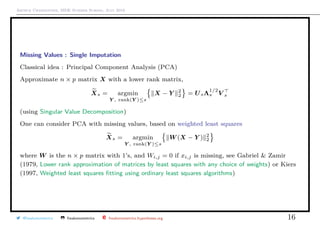
Missing Values : Single Imputation
Classical idea : Principal Component Analysis (PCA)
Approximate n × p matrix X with a lower rank matrix,
Xs = argmin
Y , rank(Y )≤s
X − Y 2
2 = UsΛ
1/2
s V s
(using Singular Value Decomposition)
One can consider PCA with missing values, based on weighted least squares
Xs = argmin
Y , rank(Y )≤s
W (X − Y ) 2
2
where W is the n × p matrix with 1’s, and Wi,j = 0 if xi,j is missing, see Gabriel & Zamir
(1979, Lower rank approximation of matrices by least squares with any choice of weights) or Kiers
(1997, Weighted least squares ﬁtting using ordinary least squares algorithms)

Iterative PCA
(i) if xi,j is missing, Wi,j = 0,
x1
i,j = Wi,j · x0
i,j + (1 − Wi,j) · 0
(ii) for k = 1, 2, · · ·
• Xs = argmin
Y , rank(Y )≤s
W (X − Y ) 2
2
• xk+1
i,j = Wi,j · xk
i,j + (1 − Wi,j) · xi,j
q
q
q
q
q
q
q
q
−0.5 0.0 0.5 1.0 1.5
−0.50.00.51.01.5
Connections with fixed effects model, xi,j =
s
k=1
fi,kuj,k + εi,j with εi,j ∼ N(0, σ2)
and random effects model, xi = Γzi + εi with εi ∼ N(0, σ2I) and zi ∼ N(0, I)

Iterative PCA
x1
i,j = Wi,j · x0
i,j + (1 − Wi,j) · 0
(ii) for k = 1, 2, · · ·
• Xs = argmin
Y , rank(Y )≤s
W (X − Y ) 2
2
• xk+1
i,j = Wi,j · xk
i,j + (1 − Wi,j) · xi,j
q
q
q
q
q
q
q
q
−0.5 0.0 0.5 1.0 1.5
−0.50.00.51.01.5
q
q
s
k=1

Iterative PCA
x1
i,j = Wi,j · x0
i,j + (1 − Wi,j) · 0
(ii) for k = 1, 2, · · ·
• Xs = argmin
Y , rank(Y )≤s
W (X − Y ) 2
2
• xk+1
i,j = Wi,j · xk
i,j + (1 − Wi,j) · xi,j q
q
q
q
q
q
q
q
q
q
−0.5 0.0 0.5 1.0 1.5
−0.50.00.51.01.5
q
q
q
q
s
k=1

Iterative PCA
x1
i,j = Wi,j · x0
i,j + (1 − Wi,j) · 0
(ii) for k = 1, 2, · · ·
• Xs = argmin
Y , rank(Y )≤s
W (X − Y ) 2
2
• xk+1
i,j = Wi,j · xk
i,j + (1 − Wi,j) · xi,j q
q
q
q
q
q
q
q
q
q
−0.5 0.0 0.5 1.0 1.5
−0.50.00.51.01.5
q
q
s
k=1

The iterative PCA is simply using EM on ﬁxed eﬀects model,
xi,j =
s
i=1
fi,jui,j + εi,j with εi,j ∼ N(0, σ2
)
X
n×p
= F
n×s
U
p×s
Log-likelihood is here
log L(F , u, σ2
) = −
np
2
log 2πσ2
−
1
2σ2
X − F u 2
E step : compute E Xi,j X, F k, Uk, σ2
k (imputation)
M step : maximize the log-likelihood
Uk+1 = Xk F k F k F k
−1
and F k+1 = XkUk Uk Uk
−1

One can use regularized iterative PCA. So far, we used (SVD) XsUsΛ
1/2
s V s
Xi,j =
s
k=1
λkUi,kVj,k
Following Efron & Morris (1972, Limiting the Risk of Bayes and Empirical Bayes Estimators)
consider a shrinkage version
Xi,j =
s
k=1
λk − σ2
λk
λkUi,kVj,k =
s
k=1
λk −
σ2
λk
Ui,kVj,k
where σ2
=
n[λs + 1 + · · · + λp]
np − p − ns − ps + s2 + s
See package missMDA

One can use soft-thresholding PCA. Following Hastie & Mazumber (2015, Matrix Completion
and Low-Rank SVD)
Xi,j =
s
k=1
λk − λ
+
Ui,kVj,k
solution of
Xs = argmin
Y , rank(Y )≤s
W (X − Y ) 2
2 + λ Y
where the penalty is based on the nuclear norm (sum of the singular values).
Complicated to select λ...
See package softImpute

One can also use k-nearest neigbors
with missMDA::imputePCA(y,ncp=1) and VIM::kNN(y,k=5)

Missing Values : Multiple Imputation
It aims to allow for the uncertainty about the missing data by creating several diﬀerent
plausible imputed data sets (via Sterne et al. (2009, Multiple imputation for missing data)
Reference, Rubin (2007, Multiple imputation for nonresponse in surveys)
The idea is to generate N possible values for each missing value, see Honaker, King & Blackwell
(2010, Amelia) and library Amelia using boostrap samples or van Buuren (2018, Multivariate
Imputation by Chained Equations) with mice using bootstrap and regression
The idea of imputation is both seductive and dangerous. It is seductive because it can lull the
user into the pleasurable state of believing that the data are complete after all, and it is
dangerous because it lumps together situations where the problem is suﬃciently minor that it
can be legitimately handled in this way and situations where standard estimators applied to the
real and imputed data have substantial biases Dempster & Rubin (1983, Incomplete Data in
Sample Surveys)

Missing Values : Gaussian process regression (and krigging)
Extrapolation or interpolation ?
x y
1 y1
2 y2
3 ?
x y
1 y1
2 ?
3 y3



y1
y2
y3


 ∼ N


0,



σ1,1 σ1,2 σ1,3
σ2,1 σ2,2 σ2,3
σ3,1 σ3,2 σ3,3






y
y
∼ N 0,
Σ Σ
Σ Σ
(y |y) ∼ N(µy, Σy) where
µy = Σ Σ−1y
Σy = Σ − Σ Σ−1Σ
see Roberts et al. (2012, Gaussian Processes for Time Series) or Rasmussen & Williams (2006,
Gaussian Processes for Machine Learning)

Side 2019 #9

More Related Content

What's hot

Similar to Side 2019 #9

More from Arthur Charpentier

Recently uploaded

Side 2019 #9