The document provides a comprehensive overview of computational information geometry, focusing on its applications in image and signal processing. It discusses key concepts such as Fisher information, Bregman divergence, and various distance measures in probability manifolds, along with the exploration of geometrical structures related to statistical models. Additionally, it emphasizes the importance of understanding relationships between distances and geometries for developing efficient algorithms in this field.

1. Computational Information Geometry:
A quick review
Frank Nielsen
École Polytechnique
Sony Computer Science Laboratories, Inc
ICMS International Center for Mathematical Sciences
Edinburgh, Sep. 21-25, 2015
Computational information geometry for image and signal processing
c 2015 Frank Nielsen 1

2. 2nd Geometric Science of Information : 28-30 Oct. 2015
École Polytechnique, Palaiseau, France
www.gsi2015.org
756 p., http://www.springer.com/us/book/9783319250397
c 2015 Frank Nielsen 2

3. Geometrizing sets of parametric/non-parametric models
Model interpreted as a Point
Geometry should encapsulates model semantic and model
proximities...
Originally started with population spaces (1930, 1945)
Geometry?
neighborhood (topology, convergence)
geodesics/projection/orthogonality (dierential geometry)
invariance
Information?
data aggregation (statistics)
lossless information compression for a task (task suciency)
Fisher information
Computation?
need closed form formula or approximation/estimation
geometric predicates
c 2015 Frank Nielsen 3

4. Some time ago in 2007...
http://www.sonycsl.co.jp/person/nielsen/FrankNielsen-distances-figs.pdf
c 2015 Frank Nielsen 4

5. More recently...
If (P : Q) = p(x)f (q(x)
p(x) dν(x)
BF (P : Q) = F(P) − F(Q) − P − Q, ∇F(Q)
tBF (P : Q) = BF (P :Q)
√
1+ ∇F (Q) 2
CD,g(P : Q) = g(Q)D(P : Q)
BF,g(P : Q; W) = WBF
P
Q : Q
W
Dv
(P : Q) = D(v(P) : v(Q))
v-Divergence Dv
total Bregman divergence tB(· : ·) Bregman divergence BF (· : ·)
conformal divergence CD,g(· : ·)
Csisz´ar f-divergence If (· : ·)
scaled Bregman divergence BF (· : ·; ·)
scaled conformal divergence CD,g(· : ·; ·)
Dissimilarity measure
Divergence
c 2015 Frank Nielsen 5

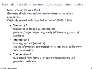
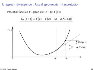
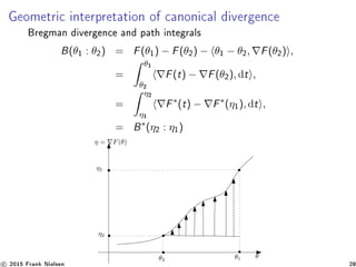
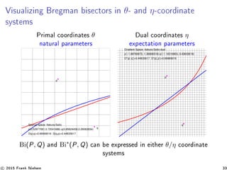
6. Programme for Computational Information Geometry
1. understand the dictionary of distances (similarities in IR,
kernels in ML, ...) and group them axiomatically into
exhaustive classes, propose new classes of
distances [6, 21, 18], and generic algorithms
2. understand relationships between distances and geometries
3. understand generalized cross/relative entropies and their
induced geometries and distributions (beyond
Shannon/Boltzmann/Gibbs)
4. provide coordinate-free intrinsic computing for applications
c 2015 Frank Nielsen 6

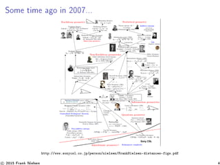
7. Cornerstone : Fisher information I(θ) = Variance of the
score
Amount of information that an observable random variable X
carries about an unknown parameter θ :
I(θ)[Ii,j ], Ii,j (θ) = Eθ[∂i l(x; θ)∂j l(x; θ)] , I(θ) 0
with (l; θ) = log p(x; θ), ∂i l(x; θ) = ∂
∂θi
l(x; θ). Cramèr-Rao bound
for variance of an estimator.
Important problem : When Fisher information is only positive
semi-denite, we have degenerate/singular models
c 2015 Frank Nielsen 7

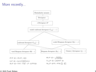
8. Fisher Information Matrix (FIM) : Our usual test friends!
I(θ) = [Ii,j (θ)]i,j , Ii,j (θ) = Eθ[∂i l(x; θ)∂j l(x; θ)]
For multinomials (p1, ..., pd ) :
I(θ) =





p1(1 − p1) −p1p2 ... −p1pk
−p1p2 p2(1 − p2) ... −p2pk
.
.
.
.
.
.
−p1pk −p2pk ... pk(1 − pk)





For multivariate normals (MVNs) N(µ, Σ) :
Ii,j (θ) =
∂µ
∂θi
Σ−1
∂µ
∂θj
+
1
2
tr Σ−1
∂Σ
∂θi
Σ−1
∂Σ
∂θj
matrix trace : tr.
c 2015 Frank Nielsen 8

9. Equivalent denitions of the Fisher information matrix
Negative expectation of the Hessian of the log-likelihood
function :
Ii,j = Eθ[∂i l(θ)∂j l(θ)]
Ii,j = 4
x
∂i p(x|θ)∂j p(x|θ)dx
Ii,j = −Eθ[∂i ∂j l(θ)]
For natural exponential families p(x|θ) = exp( θ, x − F(θ)) that
are log-concave densities
I(θ) = 2
F(θ) 0
c 2015 Frank Nielsen 9

10. Geometric structures of
probability manifolds :
(M, g, LC) Levi-Civita
metric connection
(M, g, , ∗) ⇔ (M, g, T)
Dually ane
connection ±α.
c 2015 Frank Nielsen 10

11. Dierential geometry : Orthogonality (g) and geodesics ( )
Manifold M
Riemannian manifold
metric tensor g (inner product)
(angle, orthogonality)
(M, g)
connection
covariant derivatives
⇔
parallel transport
(flatness, autoparallel)
(M, )
Levi-Civita connection
LC = (g) (coefficients Γk
ij)
geodesics preserves ·, ·
ρ(P, Q) metric distance
(shortest paths)
g ,
Differential structure (M, g, )
Dual connections (M, g, , ∗
)
c 2015 Frank Nielsen 11

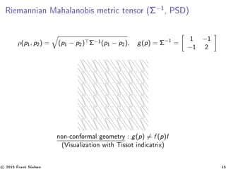
12. Riemannian geometry of population spaces
Population space : H. Hotelling [5] (1930), C. R. Rao [22] (1945)
Consider (M, g) with g = I(θ). Fisher information matrix is
unique up to a constant for statistical invariance.
Geometry of multinomials is spherical (on the orthant)
For univariate location-scale families, hyperbolic geometry or
Euclidean geometry (location only)
p(x|µ, σ) =
1
σ
p0
x − µ
σ
, X = µ + σX0
(Normal, Cauchy, Laplace, t-Student, etc.)
⇒ Studying computational hyperbolic geometry is important !
(also for computer graphics, universal covering space)
c 2015 Frank Nielsen 12

13. But rst... Distances on tangent planes = Mahalanobis
distances
Tp : tangent plane at p
Mahalanobis metric distance on tangent planes Tx :
MQ(p, q) = (p − q) Q(x)(p − q)
axioms of the metric for Q(x) = g(x) 0 (SPD).
FR distance between close points amounts to
ρ
√
2KL =
√
SKL. For exponential families,
ρ Mahalanobis = ∆θ I(θ)∆θ.
c 2015 Frank Nielsen 13

14. Extrinsic Computational Geometry on tangent planes
Tensor g = Q(x) 0 denes smooth inner product
p, q x = (p − q) Q(x)(p − q) that induces a normed
distance : dx (p, q) = p − q x = (p − q) Q(x)(p − q)
Mahalanobis metric distance on tangent planes :
∆Σ(X1, X2) = (µ1 − µ2) Σ−1
(µ1 − µ2) = ∆µ Σ−1
∆µ
Cholesky decomposition Σ = LL , lower triangular matrix L :
∆(X1, X2) = DE (L−1
µ1, L−1
µ2)
Computing on tangent planes = Euclidean computing
on transformed points x ← L−1
x.
Extrinsic vs intrinsic computations.
⇒ Reduces to usual computational geometry
c 2015 Frank Nielsen 14

15. Riemannian Mahalanobis metric tensor (Σ−1
, PSD)
ρ(p1, p2) = (p1 − p2) Σ−1
(p1 − p2), g(p) = Σ−1
=
1 −1
−1 2
non-conformal geometry : g(p) = f (p)I
(Visualization with Tissot indicatrix)
c 2015 Frank Nielsen 15

16. Normal/Gaussian family and 2D location-scale families
FIM Eθ[∂i l∂j l] for univariate normal/multivariate spherical
distributions :
I(µ, σ) =
1
σ2 0
0
2
σ2
=
1
σ2
1 0
0 2
I(µ, σ) = diag 1
σ2
, ...,
1
σ2
,
2
σ2
→ amount to Poincaré metric
dx2+dy2
y2 , hyperbolic geometry in
upper half plane/space.
c 2015 Frank Nielsen 16

17. Riemannian Klein disk metric tensor (non-conformal)
recommended for computing space since geodesics are
straight line segments (extend to Cayley-Klein spaces)
Klein is also conformal at the origin (so we can perform
translation from and back to the origin via Möbius transform.)
Geodesics passing through O in the Poincaré disk are straight
(so we can perform translation from and back to the origin)
c 2015 Frank Nielsen 17

18. A toy problem : Finding closest distributions
Given n univariate normals Ni = N(µi , σ2
i )
θi
, nd the closest
pair of distributions :
arg min
i=j
ρ(θi , θj )
... kind the rst k-th distributions to a distribution query...
Consider the Fisher Riemannian metric (aka. Rao's distance, or
Fisher-Hotelling-Rao)
ρ(Ni , Nj ) =
θj
θi
ds =
1
0
γ (t) G dt =
1
0
˙θ G(t) ˙θdt
Well, when ∀iσi = σ, ρ amounts to Euclidean distance...
How to beat the naive O(n2
) quadratic algorithm in general ?
c 2015 Frank Nielsen 18

19. Euclidean (ordinary) Voronoi diagrams
P = {P1, ..., Pn} : n distinct point generators in Euclidean space
Ed
V (Pi ) = {X : DE (Pi , X) ≤ DE (Pj , X), ∀j = i}
Voronoi diagram = cell complex V (Pi )'s with their facesc 2015 Frank Nielsen 19

20. Voronoi diagrams from bisectors and ∩ halfspaces
Bisectors
Bi(P, Q) = {X : DE (P, X) = DE (Q, X)}
→ are hyperplanes in Euclidean geometry
Voronoi cells as halfspace intersections :
V (Pi ) = {X : DE (Pi , X) ≤ DE (Pj , X), ∀j = i} = ∩n
i=1
Bi+
(Pi , Pj )
c 2015 Frank Nielsen 20

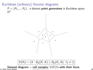
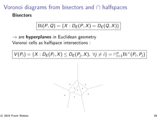
21. Voronoi diagrams and dual Delaunay simplicial complex
Empty sphere property, max min angle triangulation, etc
Voronoi dual Delaunay triangulation
→ non-degenerate point set = no (d + 2) points co-spherical
Duality : Voronoi k-face ⇔ Delaunay (d − k)-simplex
Bisector Bi(P, Q) perpendicular ⊥ to segment [PQ]
c 2015 Frank Nielsen 21

22. Mahalanobis Voronoi diagrams on tangent planes (extrinsic)
In statistics, covariance matrix Σ account for both correlation and
dimension (feature) scaling
⇔
Dual structure ≡ anisotropic Delaunay triangulation
⇒ empty circumellipse property (Cholesky decomposition)
c 2015 Frank Nielsen 22

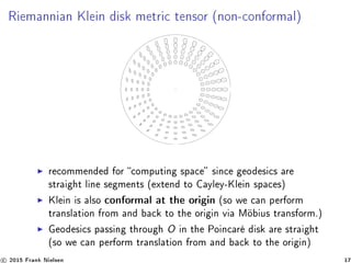
23. Hyperbolic Voronoi (Klein ane) diagrams [15, 17]
Hyperbolic Voronoi diagram in Klein disk = clipped power diagram.
Power distance :
x − p 2
− wp
→ additively weighted ordinary Voronoi = ordinary CG
c 2015 Frank Nielsen 23

24. Hyperbolic Voronoi diagrams [15, 17]
5 common models of the abstract hyperbolic geometry
https://www.youtube.com/watch?v=i9IUzNxeH4o
(5 min. video)
ACM Symposium on Computational Geometry (SoCG'14)
c 2015 Frank Nielsen 24

25. Voronoi in dually at
space : ±1-connection
instead of Levi-Civita
0-connection
c 2015 Frank Nielsen 25

26. Dually at manifolds from a convex function F
Canonical geometry induced by strictly convex and dierentiable
convex function F.
Potential functions : F and Legendre convex conjugate
G = F∗
Dual coordinate systems : θ = F∗(η) and η = F(θ).
Metric tensor g : written equivalently using the two coordinate
systems :
gij (θ) =
∂2
∂θi ∂θj
F(θ), gij
(η) =
∂2
∂ηi ∂ηj
G(η)
Divergence from Young's inequality of convex conjugates :
D(P : Q) = F(θ(P)) + F∗
(η(Q)) − θ(P), η(Q) ≥ 0
This is a Bregman divergence in disguise - :) ...
exponential family : p(x|θ) = exp( θ, x − F(θ))
Terminology : F=cumulant function, G=negative entropy
c 2015 Frank Nielsen 26

27. Bregman divergence : Usual geometric interpretation
Potential function F, graph plot F : (x, F(x)).
DF (p : q) = F(p) − F(q) − p − q, F(q)
c 2015 Frank Nielsen 27

28. Geometric interpretation of canonical divergence
Bregman divergence and path integrals
B(θ1 : θ2) = F(θ1) − F(θ2) − θ1 − θ2, F(θ2) ,
=
θ1
θ2
F(t) − F(θ2), dt ,
=
η2
η1
F∗
(t) − F∗
(η1), dt ,
= B∗
(η2 : η1)
θ
η = F(θ)
θ2 θ1
η2
η1
c 2015 Frank Nielsen 28

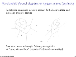
29. Statistical mixtures of exponential families
Rayleigh MMs [10] for IntraVascular UltraSound (IVUS) imaging.
log p(x|θ) = t(x), θ − F(θ) + k(x)
Rayleigh distribution :
p(x; λ) = x
λ2 e− x2
2λ2
x ∈ R+
d = 1 (univariate)
D = 1 (order 1)
θ = − 1
2λ2
Θ = (−∞, 0)
F(θ) = − log(−2θ)
t(x) = x2
k(x) = log x
(Weibull k = 2)
Coronary plaques : brotic/calcied/lipidic tissues
Rayleigh Mixture Models (RMMs) : segmentation/classication
c 2015 Frank Nielsen 29

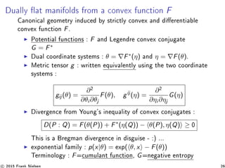
30. Dual Bregman divergences canonical divergence [14]
For P and Q belonging to the same exponential families
KL(P : Q) = EP log
p(x)
q(x)
≥ 0
= BF (θQ : θP) = BF∗ (ηP : ηQ)
= F(θQ) + F∗
(ηP) − θQ, ηP
= AF (θQ : ηP) = AF∗ (ηP : θQ)
with θQ (natural parameterization) and ηP = EP[t(X)] = F(θP)
(moment parameterization).
KL(P : Q) = p(x) log
1
q(x)
dx
H×(P:Q)
− p(x) log
1
p(x)
dx
H(p)=H×(P:P)
Shannon cross-entropy and entropy of EF [14] with k(x) = 0 :
H×
(P : Q) = F(θQ) − θQ, F(θP) − EP[k(x)]
H(P) = F(θP) − θP, F(θP) − EP[k(x)]
H(P) = −F∗
(ηP) − EP[k(x)]
c 2015 Frank Nielsen 30

31. Closed-form : algebraic vs analytic formula
Shannon cross-entropy and entropy of exponential families [14] :
H×
(P : Q) = F(θQ) − θQ, F(θP) − EP[k(x)]
H(P) = F(θP) − θP, F(θP) − EP[k(x)]
H(P) = −F∗
(ηP) − EP[k(x)]
Poisson entropy [1](1988) :
H(Poi(λ)) = λ(1 − log λ) + e−λ
∞
k=0
λk log k!
k!
Rayleigh entropy [14] :
H(Ray(σ)) = 1 + log
σ
√
2
+
γ
2
with γ the Euler-Mascheroni constant
c 2015 Frank Nielsen 31

32. Dual divergence/Bregman dual bisectors [3, 13, 16]
Bregman sided (reference) bisectors related by convex duality :
BiF (θ1, θ2) = {θ ∈ Θ |BF (θ : θ1) = BF (θ : θ1)}
BiF∗ (η1, η2) = {η ∈ H |BF∗ (η : η1) = BF∗ (η : η1)}
Right-sided bisector : → θ-hyperplane, η-hypersurface
HF (p, q) = {x ∈ X | BF (x : p ) = BF (x : q )}.
F(p) − F(q), x + (F(p) − F(q) + q, F(q) − p, F(p) ) = 0
Left-sided bisector : → θ-hypersurface, η-hyperplane
HF (p, q) = {x ∈ X | BF ( p : x) = BF ( q : x)}
HF : F(x), q − p + F(p) − F(q) = 0
hyperplane = autoparallel submanifold of dimension d − 1
c 2015 Frank Nielsen 32

33. Visualizing Bregman bisectors in θ- and η-coordinate
systems
Primal coordinates θ Dual coordinates η
natural parameters expectation parameters
Bi(P, Q) and Bi∗
(P, Q) can be expressed in either θ/η coordinate
systems
c 2015 Frank Nielsen 33

34. Application of Bregman Voronoi diagrams : Closest
Bregman pair [9, 8]
Geometry of the best error exponent for multiple hypothesis testing
(MHT)
Bayesian hypothesis testing
n-ary MHT from minimum pairwise Cherno distance :
C(P1, ..., Pn) = min
i,j=i
C(Pi , Pj )
Pm
e ≤ e−mC(Pi∗ ,Pj∗ )
, (i∗
, j∗
) = argmini,j=i C(Pi , Pj )
Compute for each pair of natural neighbors [?] Pθi
and Pθj
, the
Cherno distance C(Pθi
, Pθj
), and choose the pair with minimal
distance.
→ Closest Bregman pair problem (Cherno distance fails triangle
inequality).
c 2015 Frank Nielsen 34

35. Application of Bregman Voronoi diagrams : Minimum
pairwise Cherno information [9, 8]
pθ1
pθ2
pθ∗
12
m-bisector
e-geodesic Ge(Pθ1
, Pθ2
)
(a) (b)
η-coordinate system
Pθ∗
12
C(θ1 : θ2) = B(θ1 : θ∗
12)
Bim(Pθ1
, Pθ2
)
Chernoff distribution between
natural neighbours
c 2015 Frank Nielsen 35

36. Spaces of spheres :
1-to-1 mapping between
d-spheres and
(d + 1)-hyperplanes using
potential functions
c 2015 Frank Nielsen 36

37. Space of Bregman spheres and Bregman balls [3]
Dual sided Bregman balls (bounding Bregman spheres) :
Ballr
F (c, r) = {x ∈ X | BF (x : c) ≤ r}
Balll
F (c, r) = {x ∈ X | BF (c : x) ≤ r}
Legendre duality :
Balll
F (c, r) = ( F)−1
(Ballr
F∗ ( F(c), r))
Illustration for Itakura-Saito divergence, F(x) = − log x
c 2015 Frank Nielsen 37

38. Lifting/Polarity : Potential function graph F
c 2015 Frank Nielsen 38

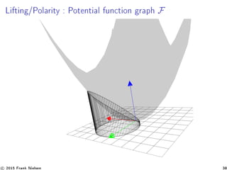
39. Space of Bregman spheres : Lifting map [3]
F : x → ˆx = (x, F(x)), hypersurface in Rd+1
, potential function
Hp : Tangent hyperplane at ˆp
z = Hp(x) = x − p, F(p) + F(p)
Bregman sphere σ −→ ˆσ with supporting hyperplane
Hσ : z = x − c, F(c) + F(c) + r.
(// to Hc and shifted vertically by r)
ˆσ = F ∩ Hσ.
intersection of any hyperplane H with F projects onto X as a
Bregman sphere :
H : z = x, a +b → σ : BallF (c = ( F)−1
(a), r = a, c −F(c)+b)
c 2015 Frank Nielsen 39

40. Space of Bregman spheres : Algorithmic applications [3]
Vapnik-Chervonenkis dimension (VC-dim) is d + 1 for the class
of Bregman balls (for Machine Learning).
Union/intersection of Bregman d-spheres from
representational (d + 1)-polytope [3]
Radical axis of two Bregman balls is an hyperplane :
Applications to Nearest Neighbor search trees like Bregman
ball trees or Bregman vantage point trees [19].
c 2015 Frank Nielsen 40

41. Bregman proximity data structures [19], k-NN queries
Vantage point trees : partition space according to Bregman balls
Partitionning space with intersection of Kullback-Leibler balls
→ ecient nearest neighbour queries in information spaces
c 2015 Frank Nielsen 41

42. Application : Minimum Enclosing Ball [12, 20]
To a hyperplane Hσ = H(a, b) : z = a, x +b in Rd+1
, corresponds
a ball σ = Ball(c, r) in Rd with center c = F∗(a) and radius :
r = a, c −F(c)+b = a, F∗
(a) −F( F∗
(a))+b = F∗
(a) + b
since F( F∗(a)) = F∗(a), a − F∗(a) (Young equality)
SEB : Find halfspace H(a, b)− : z ≤ a, x + b that contains all
lifted points :
min
a,b
r = F∗
(a) + b,
∀i ∈ {1, ..., n}, a, xi + b − F(xi ) ≥ 0
→ Convex Program (CP) with linear inequality constraints
F(θ) = F∗(η) = 1
2
x x : CP → Quadratic Programming
(QP) [4] used in SVM. Smallest enclosing ball used as a
primitive in SVM [23]
c 2015 Frank Nielsen 42

43. Approximating the smallest Bregman enclosing balls [20, 11]
Algorithm 1: BBCA(P, l).
c1 ← choose randomly a point in P;
for i = 2 to l − 1 do
// farthest point from ci wrt. BF
si ← argmaxn
j=1
BF (ci : pj );
// update the center: walk on the η-segment [ci , psi ]η
ci+1 ← F−1
( F(ci )# 1
i+1
F(psi )) ;
end
// Return the SEBB approximation
return Ball(cl , rl = BF (cl : X)) ;
θ-, η-geodesic segments in dually at geometry.
c 2015 Frank Nielsen 43

44. Smallest enclosing balls : Core-sets [20]
Core-set C ⊆ S : SOL(S) ≤ SOL(C) ≤ (1 + )SOL(S)
extended Kullback-Leibler Itakura-Saito
c 2015 Frank Nielsen 44

45. Programming InSphere predicates [3]
Implicit representation of Bregman spheres/balls : consider d + 1
support points on the boundary
Is x inside the Bregman ball dened by d + 1 support points?
InSphere(x; p0, ..., pd ) =
1 ... 1 1
p0 ... pd x
F(p0) ... F(pd ) F(x)
sign of a (d + 2) × (d + 2) matrix determinant
InSphere(x; p0, ..., pd ) is negative, null or positive depending
on whether x lies inside, on, or outside σ.
c 2015 Frank Nielsen 45

46. Smallest enclosing ball in Riemannian manifolds [2]
c = a#M
t b : point γ(t) on the geodesic line segment [ab] wrt M
such that ρM(a, c) = t × ρM(a, b) (with ρM the metric distance on
manifold M)
Algorithm 2: GeoA
c1 ← choose randomly a point in P;
for i = 2 to l do
// farthest point from ci
si ← argmaxn
j=1
ρ(ci , pj );
// update the center: walk on the geodesic line
segment [ci , psi ]
ci+1 ← ci #M
1
i+1
psi ;
end
// Return the SEB approximation
return Ball(cl , rl = ρ(cl , P)) ;
c 2015 Frank Nielsen 46

47. Computing f -divergences
for generic f :
Beyond stochastic
Monte-Carlo numerical
integration
c 2015 Frank Nielsen 47

48. Ali-Silvey-Csiszár f -divergences [7]
If (X1 : X2) = x1(x)f
x2(x)
x1(x)
dν(x) ≥ 0 (potentially +∞)
Name of the f -divergence Formula If (P : Q) Generator f (u) with f (1) = 0
Total variation (metric) 1
2 |p(x) − q(x)|dν(x) 1
2 |u − 1|
Squared Hellinger ( p(x) − q(x))2dν(x) (
√
u − 1)2
Pearson χ2
P
(q(x)−p(x))2
p(x)
dν(x) (u − 1)2
Neyman χ2
N
(p(x)−q(x))2
q(x)
dν(x)
(1−u)2
u
Pearson-Vajda χk
P
(q(x)−λp(x))k
pk−1(x)
dν(x) (u − 1)k
Pearson-Vajda |χ|k
P
|q(x)−λp(x)|k
pk−1(x)
dν(x) |u − 1|k
Kullback-Leibler p(x) log p(x)
q(x)
dν(x) − log u
reverse Kullback-Leibler q(x) log q(x)
p(x)
dν(x) u log u
α-divergence 4
1−α2 (1 − p
1−α
2 (x)q1+α
(x)dν(x)) 4
1−α2 (1 − u
1+α
2 )
Jensen-Shannon 1
2 (p(x) log 2p(x)
p(x)+q(x)
+ q(x) log 2q(x)
p(x)+q(x)
)dν(x) −(u + 1) log 1+u
2 + u log u
If (p : q) =
1
n
i
f (x2(si )/x1(si )), s1, ..., sn ∼iid X1(never +∞ !)
c 2015 Frank Nielsen 48

49. Information monotonicity of f -divergences [7]
(Proof in Ali-Silvey paper)
Do coarse binning : from d bins to k d bins :
X = k
i=1
Ai
Let pA = (pi )A with pi = j∈Ai
pj .
Information monotonicity :
D(p : q) ≥ D(pA
: qA
)
We should distinguish less downgraded histograms...
⇒ f -divergences are the only divergences preserving the
information monotonicity.
c 2015 Frank Nielsen 49

50. f -divergences and higher-order Vajda χk
divergences [7]
If (X1 : X2) =
∞
k=0
f (k)(1)
k!
χk
P(X1 : X2)
χk
P(X1 : X2) =
(x2(x) − x1(x))k
x1(x)k−1
dν(x),
|χ|k
P(X1 : X2) =
|x2(x) − x1(x)|k
x1(x)k−1
dν(x),
are f -divergences for the generators (u − 1)k and |u − 1|k.
When k = 1, χ1
P(X1 : X2) = (x1(x) − x2(x))dν(x) = 0
(never discriminative), and |χ1
P|(X1, X2) is twice the total
variation distance.
χk
P is a signed distance
c 2015 Frank Nielsen 50

51. Ane exponential families [7]
Canonical decomposition of the probability measure :
pθ(x) = exp( t(x), θ − F(θ) + k(x)),
consider natural parameter space Θ ane (like multinomials).
Poi(λ) : p(x|λ) =
λx e−λ
x!
, λ 0, x ∈ {0, 1, ...}
NorI (µ) : p(x|µ) = (2π)−d
2 e−1
2 (x−µ) (x−µ)
, µ ∈ Rd
, x ∈ Rd
Family θ Θ F(θ) k(x) t(x) ν
Poisson log λ R eθ − log x! x νc
Iso.Gaussian µ Rd 1
2
θ θ d
2
log 2π − 1
2
x x x νL
c 2015 Frank Nielsen 51

52. Higher-order Vajda χk
divergences [7]
The (signed) χk
P distance between members X1 ∼ EF (θ1) and
X2 ∼ EF (θ2) of the same ane exponential family is (k ∈ N)
always bounded and equal to :
χk
P(X1 : X2) =
k
j=0
(−1)k−j k
j
eF((1−j)θ1+jθ2)
e(1−j)F(θ1)+jF(θ2)
For Poisson/Normal distributions, we get closed-form formula :
χk
P(λ1 : λ2) =
k
j=0
(−1)k−j k
j
eλ1−j
1 λj
2−((1−j)λ1+jλ2)
,
χk
P(µ1 : µ2) =
k
j=0
(−1)k−j k
j
e
1
2 j(j−1)(µ1−µ2) (µ1−µ2)
.
c 2015 Frank Nielsen 52

53. Thank you !
Applications to
clustering and learning
mixtures will be
discussed in the second
talk !
c 2015 Frank Nielsen 53

54. Bibliography I
Robert Appledorn, Ronald J Evans, and J Boersma.
The entropy of a Poisson distribution).
SIAM Review, 30(2) :314317, 1988.
Marc Arnaudon and Frank Nielsen.
On approximating the Riemannian 1-center.
Computational Geometry, 46(1) :93 104, 2013.
Jean-Daniel Boissonnat, Frank Nielsen, and Richard Nock.
Bregman Voronoi diagrams.
Discrete and Computational Geometry, 44(2) :281307, April 2010.
Bernd Gärtner and Sven Schönherr.
An ecient, exact, and generic quadratic programming solver for geometric optimization.
In Proceedings of the sixteenth annual symposium on Computational geometry, pages 110118.
ACM, 2000.
Harold Hotelling.
Meizhu Liu, Baba C. Vemuri, Shun-ichi Amari, and Frank Nielsen.
Shape retrieval using hierarchical total Bregman soft clustering.
Transactions on Pattern Analysis and Machine Intelligence, 34(12) :24072419, 2012.
F. Nielsen and R. Nock.
On the chi square and higher-order chi distances for approximating f -divergences.
Signal Processing Letters, IEEE, 21(1) :1013, 2014.
c 2015 Frank Nielsen 54

55. Bibliography II
Frank Nielsen.
Hypothesis testing, information divergence and computational geometry.
In Frank Nielsen and Frederic Barbaresco, editors, GSI, volume 8085 of Lecture Notes in
Computer Science, pages 241248. Springer, 2013.
Frank Nielsen.
An information-geometric characterization of Cherno information.
Signal Processing Letters, IEEE, 20(3) :269272, 2013.
Frank Nielsen and Vincent Garcia.
Statistical exponential families : A digest with ash cards, 2009.
arXiv.org :0911.4863.
Frank Nielsen and Richard Nock.
On approximating the smallest enclosing Bregman balls.
In Proceedings of the Twenty-second Annual Symposium on Computational Geometry, SCG '06,
pages 485486, New York, NY, USA, 2006. ACM.
Frank Nielsen and Richard Nock.
On the smallest enclosing information disk.
Information Processing Letters (IPL), 105(3) :9397, 2008.
Frank Nielsen and Richard Nock.
The dual Voronoi diagrams with respect to representational Bregman divergences.
In International Symposium on Voronoi Diagrams (ISVD), pages 7178, 2009.
Frank Nielsen and Richard Nock.
Entropies and cross-entropies of exponential families.
In International Conference on Image Processing (ICIP), pages 36213624, 2010.
c 2015 Frank Nielsen 55

56. Bibliography III
Frank Nielsen and Richard Nock.
Hyperbolic Voronoi diagrams made easy.
In 2013 13th International Conference on Computational Science and Its Applications, pages
7480. IEEE, 2010.
Frank Nielsen and Richard Nock.
Hyperbolic Voronoi diagrams made easy.
In International Conference on Computational Science and its Applications (ICCSA), volume 1,
pages 7480, Los Alamitos, CA, USA, march 2010. IEEE Computer Society.
Frank Nielsen and Richard Nock.
Visualizing hyperbolic Voronoi diagrams.
In Symposium on Computational Geometry, page 90, 2014.
Frank Nielsen and Richard Nock.
Total Jensen divergences : Denition, properties and clustering.
In IEEE International Conference on Acoustics, Speech and Signal Processing (ICASSP), 2015.
Frank Nielsen, Paolo Piro, and Michel Barlaud.
Bregman vantage point trees for ecient nearest neighbor queries.
In Proceedings of the 2009 IEEE International Conference on Multimedia and Expo (ICME),
pages 878881, 2009.
Richard Nock and Frank Nielsen.
Fitting the smallest enclosing Bregman ball.
In Machine Learning, volume 3720 of Lecture Notes in Computer Science, pages 649656.
Springer Berlin Heidelberg, 2005.
Richard Nock, Frank Nielsen, and Shun-ichi Amari.
On conformal divergences and their population minimizers.
CoRR, abs/1311.5125, 2013.
c 2015 Frank Nielsen 56

57. Bibliography IV
Calyampudi Radhakrishna Rao.
Information and the accuracy attainable in the estimation of statistical parameters.
Bulletin of the Calcutta Mathematical Society, 37 :8189, 1945.
Ivor W. Tsang, Andras Kocsor, and James T. Kwok.
Simpler core vector machines with enclosing balls.
In Proceedings of the 24th International Conference on Machine Learning (ICML), pages
911918, New York, NY, USA, 2007. ACM.
c 2015 Frank Nielsen 57