Download to read offline

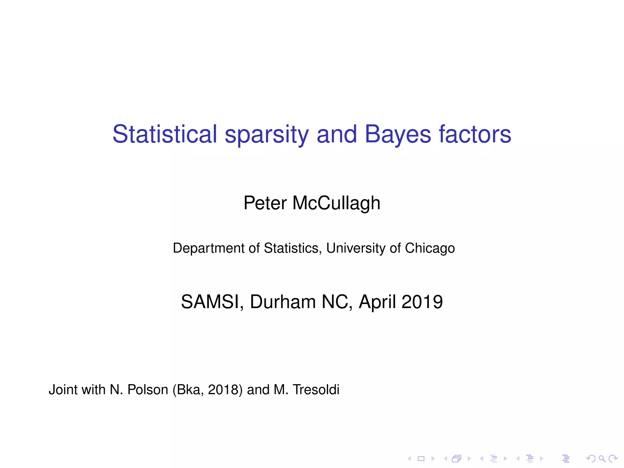
![Subset selection (to a sparse probabilist)
Need a sparse signal process X = (X1, X2, . . .)
1. X[n] = (X1, . . . , Xn) ∼ Pn,ν
2. Sparsity rate ρν, exceedance measure H = (H1, H2, . . .)
lim
ν→0
ρ−1
ν
Rn
w(x)Pn,ν(dx) =
Rn
w(x)Hn(dx)
3. Consistency:
Pn,ν(A) = Pn+1,ν(A × R) =⇒ Hn(A) = Hn+1(A × R)
4. Consistency of inverse-power measures for n = 1, 2, . . .
Hn(dx) =
Γ(n/2 + α/2)
πn/2
dx
x n+α
,
Kn =
Rn
(1 − e− x 2/2
) Hn(dx) = O(nα/2
).
5. Zeta functions
ζn(y) = K−1
n
Rn
cosh(yx) − 1 e− x 2/2
Hn(dx)](https://image.slidesharecdn.com/pmccullagh-statisticalsparsity-190430205408/85/MUMS-Bayesian-Fiducial-and-Frequentist-Conference-Statistical-Sparsity-Peter-McCullagh-April-29-2019-27-320.jpg)
![Subset selection (to a sparse probabilist)
Need a sparse signal process X = (X1, X2, . . .)
1. X[n] = (X1, . . . , Xn) ∼ Pn,ν
2. Sparsity rate ρν, exceedance measure H = (H1, H2, . . .)
lim
ν→0
ρ−1
ν
Rn
w(x)Pn,ν(dx) =
Rn
w(x)Hn(dx)
3. Consistency:
Pn,ν(A) = Pn+1,ν(A × R) =⇒ Hn(A) = Hn+1(A × R)
4. Consistency of inverse-power measures for n = 1, 2, . . .
Hn(dx) =
Γ(n/2 + α/2)
πn/2
dx
x n+α
,
Kn =
Rn
(1 − e− x 2/2
) Hn(dx) = O(nα/2
).
5. Zeta functions
ζn(y) = K−1
n
Rn
cosh(yx) − 1 e− x 2/2
Hn(dx)](https://image.slidesharecdn.com/pmccullagh-statisticalsparsity-190430205408/85/MUMS-Bayesian-Fiducial-and-Frequentist-Conference-Statistical-Sparsity-Peter-McCullagh-April-29-2019-28-320.jpg)
![Subset selection (to a sparse probabilist)
Need a sparse signal process X = (X1, X2, . . .)
1. X[n] = (X1, . . . , Xn) ∼ Pn,ν
2. Sparsity rate ρν, exceedance measure H = (H1, H2, . . .)
lim
ν→0
ρ−1
ν
Rn
w(x)Pn,ν(dx) =
Rn
w(x)Hn(dx)
3. Consistency:
Pn,ν(A) = Pn+1,ν(A × R) =⇒ Hn(A) = Hn+1(A × R)
4. Consistency of inverse-power measures for n = 1, 2, . . .
Hn(dx) =
Γ(n/2 + α/2)
πn/2
dx
x n+α
,
Kn =
Rn
(1 − e− x 2/2
) Hn(dx) = O(nα/2
).
5. Zeta functions
ζn(y) = K−1
n
Rn
cosh(yx) − 1 e− x 2/2
Hn(dx)](https://image.slidesharecdn.com/pmccullagh-statisticalsparsity-190430205408/85/MUMS-Bayesian-Fiducial-and-Frequentist-Conference-Statistical-Sparsity-Peter-McCullagh-April-29-2019-29-320.jpg)
![Subset selection (to a sparse probabilist)
Need a sparse signal process X = (X1, X2, . . .)
1. X[n] = (X1, . . . , Xn) ∼ Pn,ν
2. Sparsity rate ρν, exceedance measure H = (H1, H2, . . .)
lim
ν→0
ρ−1
ν
Rn
w(x)Pn,ν(dx) =
Rn
w(x)Hn(dx)
3. Consistency:
Pn,ν(A) = Pn+1,ν(A × R) =⇒ Hn(A) = Hn+1(A × R)
4. Consistency of inverse-power measures for n = 1, 2, . . .
Hn(dx) =
Γ(n/2 + α/2)
πn/2
dx
x n+α
,
Kn =
Rn
(1 − e− x 2/2
) Hn(dx) = O(nα/2
).
5. Zeta functions
ζn(y) = K−1
n
Rn
cosh(yx) − 1 e− x 2/2
Hn(dx)](https://image.slidesharecdn.com/pmccullagh-statisticalsparsity-190430205408/85/MUMS-Bayesian-Fiducial-and-Frequentist-Conference-Statistical-Sparsity-Peter-McCullagh-April-29-2019-30-320.jpg)
![Subset selection (to a sparse probabilist)
Need a sparse signal process X = (X1, X2, . . .)
1. X[n] = (X1, . . . , Xn) ∼ Pn,ν
2. Sparsity rate ρν, exceedance measure H = (H1, H2, . . .)
lim
ν→0
ρ−1
ν
Rn
w(x)Pn,ν(dx) =
Rn
w(x)Hn(dx)
3. Consistency:
Pn,ν(A) = Pn+1,ν(A × R) =⇒ Hn(A) = Hn+1(A × R)
4. Consistency of inverse-power measures for n = 1, 2, . . .
Hn(dx) =
Γ(n/2 + α/2)
πn/2
dx
x n+α
,
Kn =
Rn
(1 − e− x 2/2
) Hn(dx) = O(nα/2
).
5. Zeta functions
ζn(y) = K−1
n
Rn
cosh(yx) − 1 e− x 2/2
Hn(dx)](https://image.slidesharecdn.com/pmccullagh-statisticalsparsity-190430205408/85/MUMS-Bayesian-Fiducial-and-Frequentist-Conference-Statistical-Sparsity-Peter-McCullagh-April-29-2019-31-320.jpg)
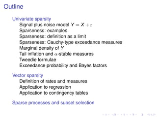
![Sparse process and subset selection (contd)
If we want a conditional distribution on subsets b ⊂ [n]
...we need a process with masses on subspaces Vb
b ⊂ [n] → Vb ⊂ Rn
; HQ
n (Vb) > 0; Pν(X ∈ Vb | Y) =???
1. Singular exceedance process...
HQ
n (dx) =
b⊂[n];b=∅
Qn(b) Hb(dx[b]) δ0(dx[¯b])
KQ
n =
Rn
(1 − e− x 2/2
)HQ
n (dx) =
b⊂[n];b=∅
Qn(b)Kb.
2. HQ is consistent if Qn(b) = Qn+1(b) + Qn+1(b ∪ {n + 1}).
e.g. Qn(b) = λ
n + λ
#b
−1
λ
#b](https://image.slidesharecdn.com/pmccullagh-statisticalsparsity-190430205408/85/MUMS-Bayesian-Fiducial-and-Frequentist-Conference-Statistical-Sparsity-Peter-McCullagh-April-29-2019-32-320.jpg)
![Sparse process and subset selection (contd)
If we want a conditional distribution on subsets b ⊂ [n]
...we need a process with masses on subspaces Vb
b ⊂ [n] → Vb ⊂ Rn
; HQ
n (Vb) > 0; Pν(X ∈ Vb | Y) =???
1. Singular exceedance process...
HQ
n (dx) =
b⊂[n];b=∅
Qn(b) Hb(dx[b]) δ0(dx[¯b])
KQ
n =
Rn
(1 − e− x 2/2
)HQ
n (dx) =
b⊂[n];b=∅
Qn(b)Kb.
2. HQ is consistent if Qn(b) = Qn+1(b) + Qn+1(b ∪ {n + 1}).
e.g. Qn(b) = λ
n + λ
#b
−1
λ
#b](https://image.slidesharecdn.com/pmccullagh-statisticalsparsity-190430205408/85/MUMS-Bayesian-Fiducial-and-Frequentist-Conference-Statistical-Sparsity-Peter-McCullagh-April-29-2019-33-320.jpg)
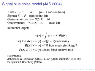
![Sparse process and subset selection (contd)
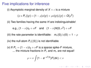
1. Marginal distribution of Y = X + ε is a mixture
mν(y) = φn(y) 1 − ρKQ
n + ρ
b⊂[n];b=∅
Qn(b) Kb ζb( y[b] )
= (1 − ρKQ
n )φn(y) + ρ
b⊂[n];b=∅
Qn(b) Kb ψ(y[b]) φ(y[¯b])
2. Conditional distribution on subsets B = {i : |Xi| > }
Pn,ν(b | Y) ∝
ρ Qn(b) Kb ζb( y[b] ) b = ∅
1 − ρKQ
n b = ∅.
3. Bayes factor for b ⊂ [n] is ζb( y[b] )](https://image.slidesharecdn.com/pmccullagh-statisticalsparsity-190430205408/85/MUMS-Bayesian-Fiducial-and-Frequentist-Conference-Statistical-Sparsity-Peter-McCullagh-April-29-2019-34-320.jpg)
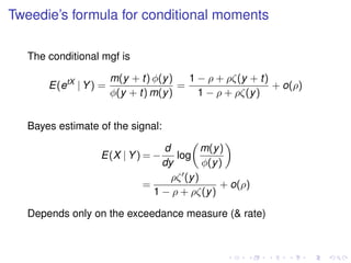
![Sparse process and subset selection (contd)
1. Marginal distribution of Y = X + ε is a mixture
mν(y) = φn(y) 1 − ρKQ
n + ρ
b⊂[n];b=∅
Qn(b) Kb ζb( y[b] )
= (1 − ρKQ
n )φn(y) + ρ
b⊂[n];b=∅
Qn(b) Kb ψ(y[b]) φ(y[¯b])
2. Conditional distribution on subsets B = {i : |Xi| > }
Pn,ν(b | Y) ∝
ρ Qn(b) Kb ζb( y[b] ) b = ∅
1 − ρKQ
n b = ∅.
3. Bayes factor for b ⊂ [n] is ζb( y[b] )](https://image.slidesharecdn.com/pmccullagh-statisticalsparsity-190430205408/85/MUMS-Bayesian-Fiducial-and-Frequentist-Conference-Statistical-Sparsity-Peter-McCullagh-April-29-2019-35-320.jpg)
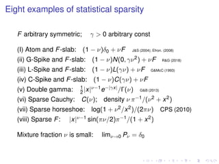
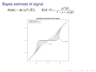
![Sparse process and subset selection (contd)
1. Marginal distribution of Y = X + ε is a mixture
mν(y) = φn(y) 1 − ρKQ
n + ρ
b⊂[n];b=∅
Qn(b) Kb ζb( y[b] )
= (1 − ρKQ
n )φn(y) + ρ
b⊂[n];b=∅
Qn(b) Kb ψ(y[b]) φ(y[¯b])
2. Conditional distribution on subsets B = {i : |Xi| > }
Pn,ν(b | Y) ∝
ρ Qn(b) Kb ζb( y[b] ) b = ∅
1 − ρKQ
n b = ∅.
3. Bayes factor for b ⊂ [n] is ζb( y[b] )](https://image.slidesharecdn.com/pmccullagh-statisticalsparsity-190430205408/85/MUMS-Bayesian-Fiducial-and-Frequentist-Conference-Statistical-Sparsity-Peter-McCullagh-April-29-2019-36-320.jpg)
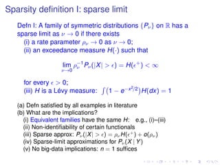
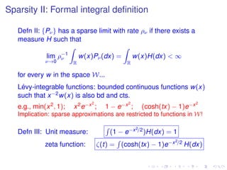
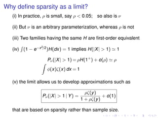
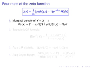
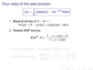
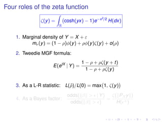
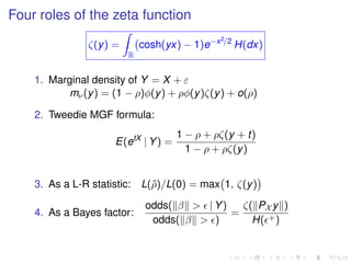
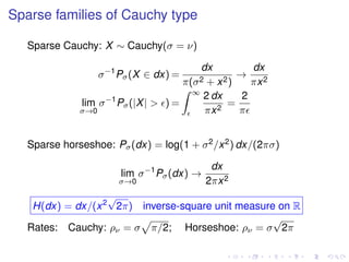
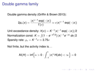
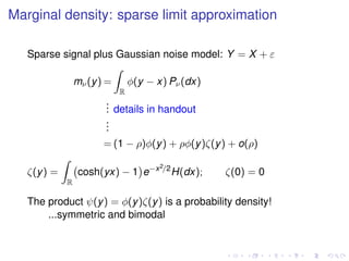
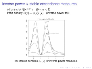
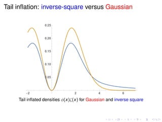
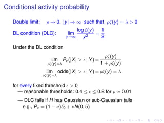
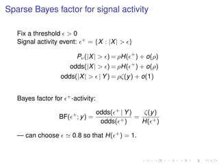
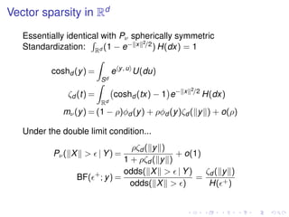
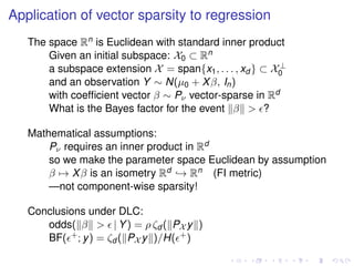
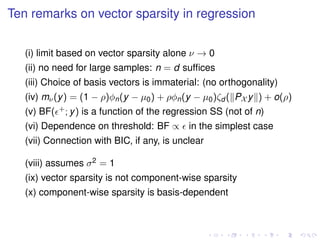
The document discusses statistical sparsity and Bayes factors, focusing on univariate and vector sparsity models, their definitions, and implications for regression analysis. It presents various examples and definitions of statistical sparsity, explores the role of the zeta function in constructing marginal densities and conditional moments, and concludes with the application of vector sparsity in regression modeling. The document emphasizes the importance of sparsity rates and their impact on inference without requiring large sample sizes.