Download as PDF, PPTX


![Arthur Charpentier, SIDE Summer School, July 2019
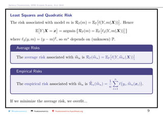
The Linear Regression
Consider some sample Sn = {(yi, xi)} where yi ∈ R and xi ∈ Rp
.
Sn is the realization of n i.i.d. random vectors (Yi, X1,i, · · · , Xp,i) with unknown
distribution P
Assume that Yi = β0 + β1x1,i + · · · + βpxp,i + εi, or Y = Xβ + ε
where εi’s satisfy E[εi] = 0, Var[εi] = σ2
, Var[εi, εj] = 0
Least square estimator of (unknown) β is
β = argmin
β∈Rp+1
y − Xβ
2
= X X
−1
X y
@freakonometrics freakonometrics freakonometrics.hypotheses.org 4](https://image.slidesharecdn.com/sidearthur2019preliminary01-190715044153/85/Side-2019-part-1-4-320.jpg)
![Arthur Charpentier, SIDE Summer School, July 2019
Geometric Perspective
Define the orthogonal projection on X,
ΠX = X[XT
X]−1
XT
y = X[XT
X]−1
X
ΠX
y = ΠXy.
Pythagoras’ theorem can be written
y 2
= ΠXy 2
+ ΠX⊥ y 2
= ΠXy 2
+ y − ΠXy 2
which can be expressed as
n
i=1
y2
i
n×total variance
=
n
i=1
y2
i
n×explained variance
+
n
i=1
(yi − yi)2
n×residual variance
@freakonometrics freakonometrics freakonometrics.hypotheses.org 5](https://image.slidesharecdn.com/sidearthur2019preliminary01-190715044153/85/Side-2019-part-1-5-320.jpg)
![Arthur Charpentier, SIDE Summer School, July 2019
Geometric Perspective
Define the angle θ between y and ΠXy,
R2
=
ΠXy 2
y 2
= 1 −
ΠX⊥ y 2
y 2
= cos2
(θ)
see Davidson & MacKinnon (2003)
y = β0 + X1β1 + X2β2 + ε
If y2 = ΠX⊥
1
y and X2 = ΠX⊥
1
X2, then
β2 = [X2
T
X2]−1
X2
T
y2
X2 = X2 if X1 ⊥ X2,
Frisch-Waugh theorem.
@freakonometrics freakonometrics freakonometrics.hypotheses.org 6](https://image.slidesharecdn.com/sidearthur2019preliminary01-190715044153/85/Side-2019-part-1-6-320.jpg)


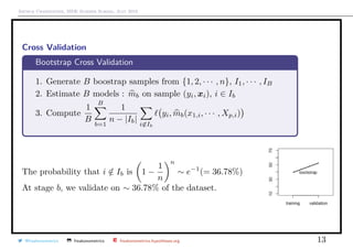
![Arthur Charpentier, SIDE Summer School, July 2019
Cross Validation
Classical Approach : split the sample Sn in two parts
Hold-Out Cross Validation
1. Split {1, 2, · · · , n} in T (training) and V (validation)
2 . Estimate m on sample (yi, xi), i ∈ T : mT
3. Compute
1
|V |
i∈V
yi, mT (x1,i, · · · , Xp,i)
1 chicago <- read.table("http:// freakonometrics .free.fr/
chicago.txt", header=TRUE ,sep=";")
2 idx <- sample (1: nrow(chicago),nrow(chicago)*.7)
3 train <- chicago[idx ,]
4 valid <- chicago[-idx ,]
@freakonometrics freakonometrics freakonometrics.hypotheses.org 10](https://image.slidesharecdn.com/sidearthur2019preliminary01-190715044153/85/Side-2019-part-1-10-320.jpg)


![Arthur Charpentier, SIDE Summer School, July 2019
Norms, Inner Products and Kernels
If H is finite, H = {h1 · · · , hd}, x, y take value Ki,j if x = hi and y = hj. Let
K = [Ki,j]
K is a symmetric d × d matrix, K = V ΛV for some orthogonal matrix V
where columns are eigenvectors, and Λ = diag[λi] (positive values). Let
Φ(x) = λ1Vi,1, λ2V2,i, · · · , λdVd,i if x = hi
Note that
Ki,j = [K = V ΛV ]i,j =
d
l=1
λlVi,lVl,j = Φ(hi), Φ(hj)
Matrix K defines an inner product, it is called a kernel. It is symmetric,
associated with a positive semi-definite matrix.
Then K(u, u) ≥ 0 and K(u, v) ≤ K(u, u) · K(v, v).
@freakonometrics freakonometrics freakonometrics.hypotheses.org 15](https://image.slidesharecdn.com/sidearthur2019preliminary01-190715044153/85/Side-2019-part-1-15-320.jpg)


![Arthur Charpentier, SIDE Summer School, July 2019
Norms, Inner Products and Kernels
Example : Consider the space H defined as
H1 = f : [0, 1] → R continuously differentiable, with f ∈ L2
([0, 1]) and f(0) = 0
H1 is an Hilbert space on [0, 1] with inner product
f, g H1
=
1
0
f (t)g (t)dt
with (definite positive) kernel K1(x, y) = min{x, y} :
f, K(x, ·) H1
=
1
0
f (t)
∂K1(t, x)
∂x
=1[0,x](t)
=
x
0
f (t)dt = f(x)
@freakonometrics freakonometrics freakonometrics.hypotheses.org 20](https://image.slidesharecdn.com/sidearthur2019preliminary01-190715044153/85/Side-2019-part-1-20-320.jpg)
![Arthur Charpentier, SIDE Summer School, July 2019
Norms, Inner Products and Kernels
Example : Consider the Sobolev space W1
([0, 1]) defined as
W1
([0, 1]) = f : [0, 1] → R continuously differentiable, with f ∈ L2
([0, 1])
Observe that W1
([0, 1]) = H0 ⊕ H1 where
H0 = f : [0, 1] → R continuously differentiable, with f = 0
The later is an Hilbert space with kernel K0(x, y) = 1.
One can consider kernel K(x, y) = K0(x, y) + K1(x, y) (related to linear splines).
More generally, consider
H2 = f : [0, 1] → R twice cont. diff., with f ∈ L2
([0, 1] with f (0) = 0)
Then f, g H2
=
1
0
f (t)g (t)dt is an inner product, with kernel
K2(x, y) =
1
0
(x − t)+(y − t)+dt
@freakonometrics freakonometrics freakonometrics.hypotheses.org 21](https://image.slidesharecdn.com/sidearthur2019preliminary01-190715044153/85/Side-2019-part-1-21-320.jpg)

![Arthur Charpentier, SIDE Summer School, July 2019
Norms, Inner Products and Kernels
Assume that yi = m(xi) + εi, where m ∈ W2([0, 1]), then polynomial splines of
degree 2 is the solution of
min
m∈W2
1
n
n
i=1
yi − m(xi)
2
+ ν
1
0
[m (t)]2
dt
then m (x) = β0 + β1x +
n
i=1
γiK2(xi, x) Note that one can use a matrix
representation
min y − Xβ − Qγ y − Xβ − Qγ + nνγ Qγ
where Q = [K1(xi, xj)]. If M = Q + nνI,
β = X M−1
X
−1
X M−1
y and γ = M−1
I−X(X M−1
X)−1
X M−1
y
@freakonometrics freakonometrics freakonometrics.hypotheses.org 23](https://image.slidesharecdn.com/sidearthur2019preliminary01-190715044153/85/Side-2019-part-1-23-320.jpg)


![Arthur Charpentier, SIDE Summer School, July 2019
How to get those kernels ?
If K1 and K2 are two kernels, so are
K(x, y) = a1K1(x, y) + a2K2(x, y) and K(x, y) = K1(x, y) · K2(x, y)
If h is some Rn
→ Rn
function, K(x, y) = K1(h(x), h(y))
If h is some Rn
→ R function, K(x, y) = h(x) · h(y)
If P is a polynomial with positive coefficients, k(x, y) = P(K1(x, y)) as well as
K(x, y) = exp[1(x, y)]
@freakonometrics freakonometrics freakonometrics.hypotheses.org 30](https://image.slidesharecdn.com/sidearthur2019preliminary01-190715044153/85/Side-2019-part-1-30-320.jpg)

The document presents a comprehensive overview of least squares in econometrics and machine learning, detailing its geometric interpretation and probabilistic approach. It covers linear regression and various cross-validation techniques to improve model validation and avoid overfitting. Additionally, it discusses norms, inner products, kernels, and the construction of reproducing kernel Hilbert spaces.