Side 2019 #3

Arthur Charpentier, SIDE Summer School, July 2019
# 3 Regularization & Penalized Regression
Arthur Charpentier (Université du Québec à Montréal)
Machine Learning & Econometrics
SIDE Summer School - July 2019
@freakonometrics freakonometrics freakonometrics.hypotheses.org 1

Linear Model and Variable Selection
Let s denote a subset of {0, 1, · · · , p}, with cardinal |s|.
Xs is the matrice with columns xj where j ∈ s.
Consider the model Y = Xsβs + η, so that βs = Xs Xs
−1
Xs y
In general, βs = (β)s
R2
is usually not a good measure since R2
(s) ≤ R2
(t) when s ⊂ t.
Some use the adjusted R2
, R
2
(s) = 1 −
n − 1
n − |s|
1 − R2
(s)
The mean square error is
mse(s) = E (Xβ − Xsβs)2
= E RSS(s) − nσ2
+ 2|s|σ2
Deﬁne Mallows’Cp as Cp(s) =
RSS(s)
σ2
− n + 2|s|
Rule of thumb: model with variables s is valid if Cp(s) ≤ |s|

In a linear model,
log L(β, σ2
) = −
n
2
log σ2
−
n
2
log(2π) −
1
2σ2
y − Xβ 2
and
log L(βs, σ2
s ) = −
n
2
log
RSS(s)
n
−
n
2
[1 + log(2π)]
It is necessary to penalize too complex models
Akaike’s AIC : AIC(s) =
n
2
log
RSS(s)
n
+
n
2
[1 + log(2π)] + 2|s|
Schwarz’s BIC : BIC(s) =
n
2
log
RSS(s)
n
+
n
2
[1 + log(2π)] + |s| log n
Exhaustive search of all models, 2p+1
... too complicated.
Stepwise procedure, forward or backward... not very stable and satisfactory.

For variable selection, use the classical stats::step function, or leaps::regsubset
for best subset, forward stepwide and backward stepwise.
For leave-one-out-cross validation, we can write
1
n
n
i=1
(yi − y(i))2
=
1
n
n
i=1
yi − yi
1 − Hi,i
2
Heuristically, (yi − yi)2
underestimates the true prediction error
High underestimation if the correlation between yi and yi is high
One can use Cov[y, y], e.g. in Mallows’ Cp,
Cp =
1
n
n
i=1
(yi − yi)2
+
2
n
σ2
p where p =
1
σ2
trace[Cov(y, y])
with Gaussian errors, AIC and Mallows’ Cp are asymptotically equivalent.

Penalized Inference and Shrinkage
Consider a parametric model, with true (unknown) parameter θ, then
mse(ˆθ) = E (ˆθ − θ)2
= E (ˆθ − E ˆθ )2
variance
+ E (E ˆθ − θ)2
bias2
One can think of a shrinkage of an unbiased estimator,
Let θ denote an unbiased estimator of θ. Then
ˆθ =
θ2
θ2 + mse(θ)
· θ = θ −
mse(θ)
θ2 + mse(θ)
· θ
penalty
satisﬁes mse(ˆθ) ≤ mse(θ).
−2 −1 0 1 2 3 4
0.00.20.40.60.8
variance

Normalization : Euclidean 2 vs. Mahalonobis
We want to penalize complicated models :
if βk is “too small”, we prefer to have βk = 0.
0.02
0.04
0.06
0.08
0.1
0.12
0.14
0.02
0.04
0.06
0.08
0.1
0.12
0.14
0.16
0.18
Instead of d(x, y) = (x − y)T
(x − y)
use dΣ(x, y) = (x − y)TΣ−1
(x − y)
beta1
beta2
beta1
beta2
−1 −0.5 0.5 1
−1
−0.5
0.5
1
30
40
40
50
60
70
80
90
100
110
120
120
150 150
X
−1.0 −0.5 0.0 0.5 1.0
−1.0−0.50.00.51.0

Linear Regression Shortcoming
Least Squares Estimator β = (XT
X)−1
XT
y
Unbiased Estimator E[β] = β
Variance Var[β] = σ2
(XT
X)−1
which can be (extremely) large when det[(XT
X)] ∼ 0.
X =







1 −1 2
1 0 1
1 2 −1
1 1 0







then XT
X =




4 2 2
2 6 −4
2 −4 6



 while XT
X+I =




5 2 2
2 7 −4
2 −4 7




eigenvalues : {10, 6, 0} {11, 7, 1}
Ad-hoc strategy: use XT
X + λI

Ridge Regression
... like the least square, but it shrinks estimated coeﬃcients towards 0.
β
ridge
λ = argmin



n
i=1
(yi − xT
i β)2
+ λ
p
j=1
β2
j



β
ridge
λ = argmin



y − Xβ
2
2
=criteria
+ λ β 2
2
=penalty



λ ≥ 0 is a tuning parameter.

Ridge Regression
an Wieringen (2018 Lecture notes on ridge regression
Ridge Estimator (OLS)
β
ridge
λ = argmin



n
i=1
(yi − xi β)2
+ λ
p
j=1
β2
j



Ridge Estimator (GLM)
β
ridge
λ = argmin



−
n
i=1
log f(yi|µi = g−1
(xi β)) +
λ
2
p
j=1
β2
j




Ridge Regression
β
ridge
λ = argmin y − (β0 + Xβ)
2
2
+ λ β
2
2
can be seen as a constrained optimization problem
β
ridge
λ = argmin
β 2
2
≤hλ
y − (β0 + Xβ)
2
2
Explicit solution
βλ = (XT
X + λI)−1
XT
y
If λ → 0, β
ridge
0 = β
ols
If λ → ∞, β
ridge
∞ = 0.
beta1
beta2
−1 −0.5 0.5 1
−1
−0.5
0.5
1
30
40
40
50
60
70
80
90
100
110
120
120
150 150
30
X
−1.0 −0.5 0.0 0.5 1.0
−1.0−0.50.00.51.0
beta1
beta2
−1 −0.5 0.5 1
−1
−0.5
0.5
1
30
40
40
50
60
70
80
90
100
110
120
120
150 150
X
−1.0 −0.5 0.0 0.5 1.0
−1.0−0.50.00.51.0

Ridge Regression
This penalty can be seen as rather unfair if compo-
nents of x are not expressed on the same scale
• center: xj = 0, then β0 = y
• scale: xT
j xj = 1
Then compute
β
ridge
λ = argmin



y − Xβ 2
2
=loss
+ λ β 2
2
=penalty



beta1
beta2
−1 −0.5 0.5 1
−1
−0.5
0.5
1
30
40
40
50
60
70
80
90
100
110
120
120
150 150
30
X
−1.0 −0.5 0.0 0.5 1.0
−1.0−0.50.00.51.0
beta1
beta2
−1 −0.5 0.5 1
−1
−0.5
0.5
1
30
40
40
50
60
70
80
90
100
110
120
120
150 150
40
40
X
−1.0 −0.5 0.0 0.5 1.0
−1.0−0.50.00.51.0

Ridge Regression
Observe that if xj1
⊥ xj2
, then
β
ridge
λ = [1 + λ]−1
β
ols
λ
which explain relationship with shrinkage.
But generally, it is not the case...
Smaller mse
There exists λ such that mse[β
ridge
λ ] ≤ mse[β
ols
λ ]
q
q

Ridge Regression
Lλ(β) =
n
i=1
(yi − β0 − xT
i β)2
+ λ
p
j=1
β2
j
∂Lλ(β)
∂β
= −2XT
y + 2(XT
X + λI)β
∂2
Lλ(β)
∂β∂βT
= 2(XT
X + λI)
where XT
X is a semi-positive deﬁnite matrix, and λI is a positive deﬁnite
matrix, and
βλ = (XT
X + λI)−1
XT
y

The Bayesian Interpretation
From a Bayesian perspective,
P[θ|y]
posterior
∝ P[y|θ]
likelihood
· P[θ]
prior
i.e. log P[θ|y] = log P[y|θ]
log likelihood
+ log P[θ]
penalty
If β has a prior N(0, τ2
I) distribution, then its posterior distribution has mean
E[β|y, X] = XT
X +
σ2
τ2
I
−1
XT
y.

Properties of the Ridge Estimator
βλ = (XT
X + λI)−1
XT
y
E[βλ] = XT
X(λI + XT
X)−1
β.
i.e. E[βλ] = β.
Observe that E[βλ] → 0 as λ → ∞.
Ridge & Shrinkage
Assume that X is an orthogonal design matrix, i.e. XT
X = I, then
βλ = (1 + λ)−1
β
ols
.

Set W λ = (I + λ[XT
X]−1
)−1
. One can prove that
W λβ
ols
= βλ.
Thus,
Var[βλ] = W λVar[β
ols
]W T
λ
and
Var[βλ] = σ2
(XT
X + λI)−1
XT
X[(XT
X + λI)−1
]T
.
Observe that
Var[β
ols
] − Var[βλ] = σ2
W λ[2λ(XT
X)−2
+ λ2
(XT
X)−3
]W T
λ ≥ 0.

Hence, the conﬁdence ellipsoid of ridge estimator is
indeed smaller than the OLS,
If X is an orthogonal design matrix,
Var[βλ] = σ2
(1 + λ)−2
I.
mse[βλ] = σ2
trace(W λ(XT
X)−1
W T
λ) + βT
(W λ − I)T
(W λ − I)β.
If X is an orthogonal design matrix,
mse[βλ] =
pσ2
(1 + λ)2
+
λ2
(1 + λ)2
βT
β
0.0 0.2 0.4 0.6 0.8
−1.0−0.8−0.6−0.4−0.2
β1
β2
1
2
3
4
5
6
7

mse[βλ] =
pσ2
(1 + λ)2
+
λ2
(1 + λ)2
βT
β
is minimal for
λ =
pσ2
βT
β
Note that there exists λ > 0 such that mse[βλ] < mse[β0] = mse[β
ols
].
Ridge regression is obtained using glmnet::glmnet(..., alpha = 0) - and
glmnet::cv.glmnet for cross validation

SVD decomposition
For any matrix A, m × n, there are orthogonal matrices U (m × m), V (n × n)
and a ”diagonal” matrix Σ (m × n) such that A = UΣV T
, or AV = UΣ.
Hence, there exists a special orthonormal set of vectors (i.e. the columns of V ),
that is mapped by the matrix A into an orthonormal set of vectors (i.e. the
columns of U).
Let r = rank(A), then A =
r
i=1
σiuivT
i (called the dyadic decomposition of A).
Observe that it can be used to compute (e.g.) the Frobenius norm of A,
A = a2
i,j = σ2
1 + · · · + σ2
min{m,n}.
Further AT
A = V ΣT
ΣV T
while AAT
= UΣΣT
UT
.
Hence, σ2
i ’s are related to eigenvalues of AT
A and AAT
, and ui, vi are associated
eigenvectors.
Golub & Reinsh (1970, Singular Value Decomposition and Least Squares Solutions)

SVD decomposition
Consider the singular value decomposition of X, X = UDV T
.
Then
β
ols
= V D−2
D UT
y
βλ = V (D2
+ λI)−1
D UT
y
Observe that
D−1
i,i ≥
Di,i
D2
i,i + λ
hence, the ridge penalty shrinks singular values.
Set now R = UD (n × n matrix), so that X = RV T
,
βλ = V (RT
R + λI)−1
RT
y

Hat matrix and Degrees of Freedom
Recall that Y = HY with
H = X(XT
X)−1
XT
Similarly
Hλ = X(XT
X + λI)−1
XT
trace[Hλ] =
p
j=1
d2
j,j
d2
j,j + λ
→ 0, as λ → ∞.

Sparsity Issues
In several applications, k can be (very) large, but a lot of features are just noise:
βj = 0 for many j’s. Let s denote the number of relevant features, with s << k,
cf Hastie, Tibshirani & Wainwright (2015, Statistical Learning with Sparsity),
s = card{S} where S = {j; βj = 0}
The model is now y = XT
SβS + ε, where XT
SXS is a full rank matrix.
q
q
= . +

Going further on sparsity issues
The Ridge regression problem was to solve
β = argmin
β∈{ β 2 ≤s}
{ Y − XT
β 2
2
}
Deﬁne a 0 = 1(|ai| > 0).
Here dim(β) = k but β 0 = s.
We wish we could solve
β = argmin
β∈{ β 0 =s}
{ Y − XT
β 2
2
}
Problem: it is usually not possible to describe all possible constraints, since
s
k
coeﬃcients should be chosen here (with k (very) large).
beta1
beta2
−1 −0.5 0.5 1
−1
−0.5
0.5
1
30
40
40
50
60
70
80
90
100
110
120
120
150 150
X
−1.0 −0.5 0.0 0.5 1.0
−1.0−0.50.00.51.0

In a convex problem, solve the dual problem,
e.g. in the Ridge regression : primal problem
min
β∈{ β 2 ≤s}
{ Y − XT
β 2
2
}
and the dual problem
min
β∈{ Y −XTβ 2 ≤t}
{ β 2
2
}
beta1
beta2
−1 −0.5 0.5 1
−1
−0.5
0.5
1
26
27
30
32
35
40
40
50
60
70
80
90
100
110
120
120
130
130
140 140
X
q
−1.0 −0.5 0.0 0.5 1.0
−1.0−0.50.00.51.0
beta1
beta2
−1 −0.5 0.5 1
−1
−0.5
0.5
1
26
27
30
32
35
40
40
50
60
70
80
90
100
110
120
120
130
130
140 140
X
q
−1.0 −0.5 0.0 0.5 1.0
−1.0−0.50.00.51.0

Idea: solve the dual problem
β = argmin
β∈{ Y −XTβ 2 ≤h}
{ β 0
}
where we might convexify the 0 norm, · 0
.

On [−1, +1]k
, the convex hull of β 0
is β 1
On [−a, +a]k
, the convex hull of β 0
is a−1
β 1
Hence, why not solve
β = argmin
β; β 1 ≤˜s
{ Y − XT
β 2 }
which is equivalent (Kuhn-Tucker theorem) to the Lagragian optimization
problem
β = argmin{ Y − XT
β 2
2
+λ β 1
}

lasso Least Absolute Shrinkage and Selection Operator
lasso Estimator (OLS)
β
lasso
λ = argmin



n
i=1
(yi − xi β)2
+ λ
p
j=1
|βj|



lasso Estimator (GLM)
β
lasso
λ = argmin



−
n
i=1
log f(yi|µi = g−1
(xi β)) +
λ
2
p
j=1
|βj|




lasso Regression
No explicit solution...
If λ → 0, β
lasso
0 = β
ols
If λ → ∞, β
lasso
∞ = 0.
beta1
beta2
−1 −0.5 0.5 1
−1
−0.5
0.5
1
30
40
40
50
60
70
80
90
100
110
120
120
150 150
X
−1.0 −0.5 0.0 0.5 1.0
−1.0−0.50.00.51.0
beta1
beta2
−1 −0.5 0.5 1
−1
−0.5
0.5
1
30
40
40
50
60
70
80
90
100
110
120
120
150 150
X
−1.0 −0.5 0.0 0.5 1.0
−1.0−0.50.00.51.0

lasso Regression
For some λ, there are k’s such that β
lasso
k,λ = 0.
Further, λ → β
lasso
k,λ is piecewise linear
beta1
beta2
−1 −0.5 0.5 1
−1
−0.5
0.5
1
30
40
40
50
60
70
80
90
100
110
120
120
150 150
30
X
−1.0 −0.5 0.0 0.5 1.0
−1.0−0.50.00.51.0
beta1
beta2
−1 −0.5 0.5 1
−1
−0.5
0.5
1
30
40
40
50
60
70
80
90
100
110
120
120
150 150
40
40
X
−1.0 −0.5 0.0 0.5 1.0
−1.0−0.50.00.51.0

lasso Regression
In the orthogonal case, XT
X = I,
β
lasso
k,λ = sign(β
ols
k ) |β
ols
k | −
λ
2
i.e. the LASSO estimate is related to the soft
threshold function...
q
q

Optimal lasso Penalty
Use cross validation, e.g. K-fold,
β(−k)(λ) = argmin



i∈Ik
[yi − xT
i β]2
+ λ β 1



then compute the sum of the squared errors,
Qk(λ) =
i∈Ik
[yi − xT
i β(−k)(λ)]2
and ﬁnally solve
λ = argmin Q(λ) =
1
K
k
Qk(λ)

Optimal lasso Penalty
Note that this might overﬁt, so Hastie, Tibshiriani & Friedman (2009, Elements
of Statistical Learning) suggest the largest λ such that
Q(λ) ≤ Q(λ ) + se[λ ] with se[λ]2
=
1
K2
K
k=1
[Qk(λ) − Q(λ)]2
lasso regression is obtained using glmnet::glmnet(..., alpha = 1) - and
glmnet::cv.glmnet for cross validation.

LASSO and Ridge, with R
1 > library(glmnet)
2 > chicago=read.table("http:// freakonometrics .free.fr/
chicago.txt",header=TRUE ,sep=";")
3 > standardize <- function(x) {(x-mean(x))/sd(x)}
4 > z0 <- standardize(chicago[, 1])
7 > ridge <-glmnet(cbind(z1 , z2), z0 , alpha =0, intercept=
FALSE , lambda =1)
8 > lasso <-glmnet(cbind(z1 , z2), z0 , alpha =1, intercept=
FALSE , lambda =1)
9 > elastic <-glmnet(cbind(z1 , z2), z0 , alpha =.5,
intercept=FALSE , lambda =1)
Elastic net, λ1 β 1 + λ2 β 2
2
q
q
q
qqqqqqqqqqqqqqqqqqqqqqqqqqqqqqqqqqqqqqqqqqqqqqqqqqqqqqqqqqqqqqqqqqqqqqqqqqqqqqqqqqqqqqqqqqqqqqqqqqqqqqqqqqqqqqqqqqqqqqqqqqqqqqqqqqqqqqqqqqqqqqqqqqqqqqqqqqqqqqqqqqqqqqqqqqqqqqqqqqqqqqqqqqqqqqqqqqq
q
q
qq
q
q
q
q
q
q
q
q
q
q
q
qqqqqqqqqqqqqqqqqqqqqqqqqqqqqqqqqqqqqqqqqqqqqqqqqqqqqqqqqqqqqqqqqqqqqqqqqqqqqqqqqqqqqqqqqqqqqqqqqqqqqqqqqqqqqqqqqqqqqqqqqqqqqqqqqqqqqqqqqqqqqqqqqqqqqqqqqqqqqqqqqqqqqqqqqqqqqqqqqqqqqqqqqqqqq
q
q
q
q
q
qq
q
q
q
q
q
qqqqqqqqqqqqqqqqqqqqqqqqqqqqqqqqqqqqqqqqqqqqqqqqqqqqqqqqqqqqqqqqqqqqqqqqqqqqqqqqqqqqqqqqqqqqqqqqqqqqqqqqqqqqqqqqqqqqqqqqqqqqqqqqqqqqqqqqqqqqqqqqqqqqqqqqqqqqqqqqqqqqqqqqqqqqqqqqqqqqqqqqqqqqq
q
q
q
q
q
q
q
q
q
q
q
qq
q
q
q
q
q

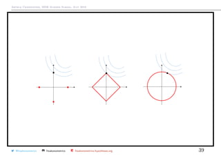
lasso and lar (Least-Angle Regression)
lasso estimation can be seen as an adaptation of LAR procedure
Least Angle Regression
(i) set (small)
(ii) start with initial residual ε = y, and β = 0
(iii) ﬁnd the predictor xj with the highest correlation with ε
(iv) update βj = βj + δj = βj + · sign[ε xj]
(v) set ε = ε − δjxj and go to (iii)
see Efron et al. (2004, Least Angle Regression)

Going further, 0, 1 and 2 penalty
Deﬁne
a 0 =
d
i=1
1(ai = 0), a 1 =
d
i=1
|ai| and a 2 =
d
i=1
a2
i
1/2
, for a ∈ Rd
.
constrained penalized
optimization optimization
argmin
β; β 0 ≤s
n
i=1
(yi, β0 + xT
β) argmin
β,λ
n
i=1
(yi, β0 + xT
β) + λ β 0 ( 0)
argmin
β; β 1 ≤s
n
i=1
(yi, β0 + xT
β) argmin
β,λ
n
i=1
(yi, β0 + xT
β) + λ β 1
( 1)
argmin
β; β 2 ≤s
n
i=1
(yi, β0 + xT
β) argmin
β,λ
n
i=1
(yi, β0 + xT
β) + λ β 2 ( 2)
Assume that is the quadratic norm.

The two problems ( 2) are equivalent : ∀(β , s ) solution of the left problem, ∃λ
such that (β , λ ) is solution of the right problem. And conversely.
The two problems ( 1) are equivalent : ∀(β , s ) solution of the left problem, ∃λ
such that (β , λ ) is solution of the right problem. And conversely. Nevertheless,
if there is a theoretical equivalence, there might be numerical issues since there is
not necessarily unicity of the solution.
The two problems ( 0) are not equivalent : if (β , λ ) is solution of the right
problem, ∃s such that β is a solution of the left problem. But the converse is
not true.
More generally, consider a p norm,
• sparsity is obtained when p ≤ 1
• convexity is obtained when p ≥ 1

Foster & George (1994) the risk inﬂation criterion for multiple regression tried to
solve directly the penalized problem of ( 0).
But it is a complex combinatorial problem in high dimension (Natarajan (1995)
sparse approximate solutions to linear systems proved that it was a NP-hard
problem)
One can prove that if λ ∼ σ2
log(p), alors
E [xT
β − xT
β0]2
≤ E [xS
T
βS − xT
β0]2
=σ2#S
· 4 log p + 2 + o(1) .
In that case
β
sub
λ,j =



0 si j /∈ Sλ(β)
β
ols
j si j ∈ Sλ(β),
where Sλ(β) is the set of non-null values in solutions of ( 0).

If is no longer the quadratic norm but 1, problem ( 1) is not always strictly
convex, and optimum is not always unique (e.g. if XT
X is singular).
But in the quadratic case, is strictly convex, and at least Xβ is unique.
Further, note that solutions are necessarily coherent (signs of coeﬃcients) : it is
not possible to have βj < 0 for one solution and βj > 0 for another one.
In many cases, problem ( 1) yields a corner-type solution, which can be seen as a
”best subset” solution - like in ( 0).

Consider a simple regression yi = xiβ + ε, with 1-penalty and a 2-loss fucntion.
( 1) becomes
min yT
y − 2yT
xβ + βxT
xβ + 2λ|β|
First order condition can be written
−2yT
x + 2xT
xβ±2λ = 0.
(the sign in ± being the sign of β). Assume that least-square estimate (λ = 0) is
(strictly) positive, i.e. yT
x > 0. If λ is not too large β and βols
have the same
sign, and
−2yT
x + 2xT
xβ + 2λ = 0.
with solution βlasso
λ =
yT
x − λ
xTx
.

Increase λ so that βλ = 0.
Increase slightly more, βλ cannot become negative, because the sign of the ﬁrst
order condition will change, and we should solve
−2yT
x + 2xT
xβ − 2λ = 0.
and solution would be βlasso
λ =
yT
x + λ
xTx
. But that solution is positive (we
assumed that yT
x > 0), to we should have βλ < 0.
Thus, at some point βλ = 0, which is a corner solution.
In higher dimension, see Tibshirani & Wasserman (2016, a closer look at sparse
regression) or Cand`es & Plan (2009, Near-ideal model selection by 1 minimization.)
With some additional technical assumption, that lasso estimator is ”sparsistent”
in the sense that the support of β
lasso
λ is the same as β,

Thus, lasso can be used for variable selection - see Hastie et al. (2001, The
Elements of Statistical Learning).
Generally, βlasso
λ is a biased estimator but its variance can be small enough to
have a smaller least squared error than the OLS estimate.
With orthonormal covariates, one can prove that
βsub
λ,j = βols
j 1|βsub
λ,j
|>b
, βridge
λ,j =
βols
j
1 + λ
and βlasso
λ,j = signe[βols
j ] · (|βols
j | − λ)+.

lasso for Autoregressive Time Series
Consider some AR(p) autoregressive time series,
Xt = φ1Xt−1 + φ2Xt−2 + · · · + φp−1Xt−p+1 + φpXt−p + εt,
for some white noise (εt), with a causal type representation. Write y = xT
φ + ε.
The lasso estimator φ is a minimizer of
1
2T
y = xT
φ 2
+ λ
p
i=1
λi|φi|,
for some tuning parameters (λ, λ1, · · · , λp).
See Nardi & Rinaldo (2011, Autoregressive process modeling via the Lasso
procedure).

lasso and Non-Linearities
Consider knots k1, · · · , km, we want a function m which is a cubic polynomial
between every pair of knots, continuous at each knot, and with ontinuous first
and second derivatives at each knot.
We can write m as
m(x) = β0 + β1x + β2x2
+ β3x3
+ β4(x − k1)3
+ + · · · + βm+3(x − km)3
+
One strategy is the following
• fix the number of knots m (m < n)
• find the natural cubic spline m which minimizes
n
i=1
(yi − m(xi))2
• then choose m by cross validation
and alternative is to use a penalty based approach (Ridge type) to avoid overfit
(since with m = n, the residual sum of square is null).

GAM, splines and Ridge regression
Consider a univariate nonlinear regression problem, so that E[Y |X = x] = m(x).
Given a sample {(y1, x1), · · · , (yn, xn)}, consider the following penalized problem
m = argmin
m∈C2
n
i=1
(yi − m(xi))2
+ λ
R
m (x)dx
with the Residual sum of squares on the left, and a penalty for the roughness of
the function.
The solution is a natural cubic spline with knots at unique values of x (see
Eubanks (1999, Nonparametric Regression and Spline Smoothing)
Consider some spline basis {h1, · · · , hn}, and let m(x) =
n
i=1
βihi(x).
Let H and Ω be the n × n matrices Hi,j = hj(xi), and Ωi,j =
R
hi (x)hj (x)dx.

Then the objective function can be written
(y − Hβ)T
(y − Hβ) + λβT
Ωβ
Recognize here a generalized Ridge regression, with solution
βλ = HT
H + λΩ
−1
HT
y.
Note that predicted values are linear functions of the observed value since
y = H HT
H + λΩ
−1
HT
y = Sλy,
with degrees of freedom trace(Sλ).
One can obtain the so-called Reinsch form by considering the singular value
decomposition of H = UDV T
.

Here U is orthogonal since H is square (n × n), and D is here invertible. Then
Sλ = (I + λUT
D−1
V T
ΩV D−1
U)−1
= (I + λK)−1
where K is a positive semideﬁnite matrix, K = B∆BT
, where columns of B are
know as the Demmler-Reinsch basis.
In that (orthonormal) basis, Sλ is a diagonal matrix,
Sλ = B I + λ∆
−1
BT
Observe that SλBk =
1
1 + λ∆k,k
Bk.
Here again, eigenvalues are shrinkage coeﬃcients of basis vectors.
With more covariates, consider an additive problem
(h1, · · · , hp) =
h1,··· ,hp∈C2
argmin



n
i=1

yi −
p
j=1
m(xi,j)


2
+ λ
p
j=1 R
mj (x)dx




which can be written
min



(y −
p
j=1
Hjβj)T
(y −
p
j=1
Hjβj) + λ β1
T
p
j=1
Ωjβj



where each matrix Hj is a Demmler-Reinsch basis for variable xj.
Chouldechova & Hastie (2015, Generalized Additive Model Selection)
Assume that the mean function for the jth variable is mj(x) = αjx + mj(x)T
βj.
One can write
min (y − α0 −
p
j=1
αjxj −
p
j=1
Hjβj)T
(y − α0 −
p
j=1
αjxj −
p
j=1
Hjβj)
+λ γ|α1| + (1 − γ) βj Ωj + ψ1β1
T
Ω1β1 + · · · + ψpβp
T
Ωpβp
where βj Ωj
= βj
TΩjβj.

The second term is the selection penalty, with a mixture of 1 and 2 (type)
norm-based penalty
The third term is the end-to-path penalty (GAM type when λ = 0).
For each predictor xj, there are three possibilities
• zero, αj = 0 and βj = 0
• linear, αj = 0 and βj = 0
• nonlinear, βj = 0

0.0 0.2 0.4 0.6 0.8
−30−101030
variable 1
smoothfunction
10 20 30 40 50 60 70
−30−101030
variable 2
smoothfunction
5 10 15 20
−30−101030
variable 3
smoothfunction
50 20 10 5 2 1
−30−20−10010
Linear Components
λ
α
50 20 10 5 2 1
05102030
Non−linear Components
λ
||β||
0 1 2 3 4
30507090
log(Lambda)
Mean−SquaredError
q
qqq
q
q
qq
q
q
q
q
q
q
q
q
qqqqqqqqqqqqqqqqqqqqqqqqqqqqqqqqqq
3 3 3 3 3 3 3 3 3 2 2 2 2 2 2 2 1
42 27
0.0 0.2 0.4 0.6 0.8
−50510
v1
f(v1)
10 20 30 40 50 60 70
−50510
v2
f(v2)
5 10 15 20
−50510
v3
f(v3)@freakonometrics freakonometrics freakonometrics.hypotheses.org 50

Coordinate Descent
LASSO Coordinate Descent Algorithm
1. Set β0 = β
2 . For k = 1, · · ·
for j = 1, · · · , p
(i) compute Rj = xj y − X−jβk−1(−j)
(ii) set βk,j = Rj · 1 −
λ
2|Rj| +
3. The ﬁnal estimate βκ is βλ

From LASSO to Dantzig Selection
Cand`es & Tao (2007, The Dantzig selector: Statistical estimation when p is much
larger than n) deﬁned
β
dantzig
λ ∈ argmin
β∈Rp
β 1
s.t. X (y − Xβ) ∞
≤ λ

From LASSO to Adaptative Lasso
Zou (2006, The Adaptive Lasso)
β
a-lasso
λ ∈ argmin
β∈Rp



y − Xβ 2
2
+ λ
p
j=1
|βj|
|βγ-lasso
λ,j |



where β
γ-lasso
λ = ΠXs(λ)
y where s(λ) is the set of non null components β
lasso
λ
See library lqa or lassogrp

From LASSO to Group Lasso
Assume that variables x ∈ Rp
can be grouped in L subgroups, x = (x1 · · · , xL),
where dim[xl] = pl.
Yuan & Lin (2007, Model selection and estimation in the Gaussian graphical model)
deﬁned, for some Kl matrices nl × nl deﬁnite positives
β
g-lasso
λ ∈ argmin
β∈Rp
y − Xβ 2
2
+ λ
L
l=1
βl Klβl
or, if Kl = plI
β
g-lasso
λ ∈ argmin
β∈Rp
y − Xβ 2
2
+ λ
L
l=1
pl βl 2
See library gglasso

From LASSO to Sparse-Group Lasso
Assume that variables x ∈ Rp
can be grouped in L subgroups, x = (x1 · · · , xL),
where dim[xl] = pl.
Simon et al. (2013, A Sparse-Group LASSO) deﬁned, for some Kl matrices nl × nl
deﬁnite positives
β
sg-lasso
λ,µ ∈ argmin
β∈Rp
y − Xβ 2
2
+ λ
L
l=1
βl Klβl + µ β 1
See library SGL

Side 2019 #3

More Related Content

What's hot

Similar to Side 2019 #3

More from Arthur Charpentier

Recently uploaded

Side 2019 #3