Side 2019 #6

Arthur Charpentier, SIDE Summer School, July 2019
# 6 Classification & Support Vector Machine
Arthur Charpentier (Université du Québec à Montréal)
Machine Learning & Econometrics
SIDE Summer School - July 2019
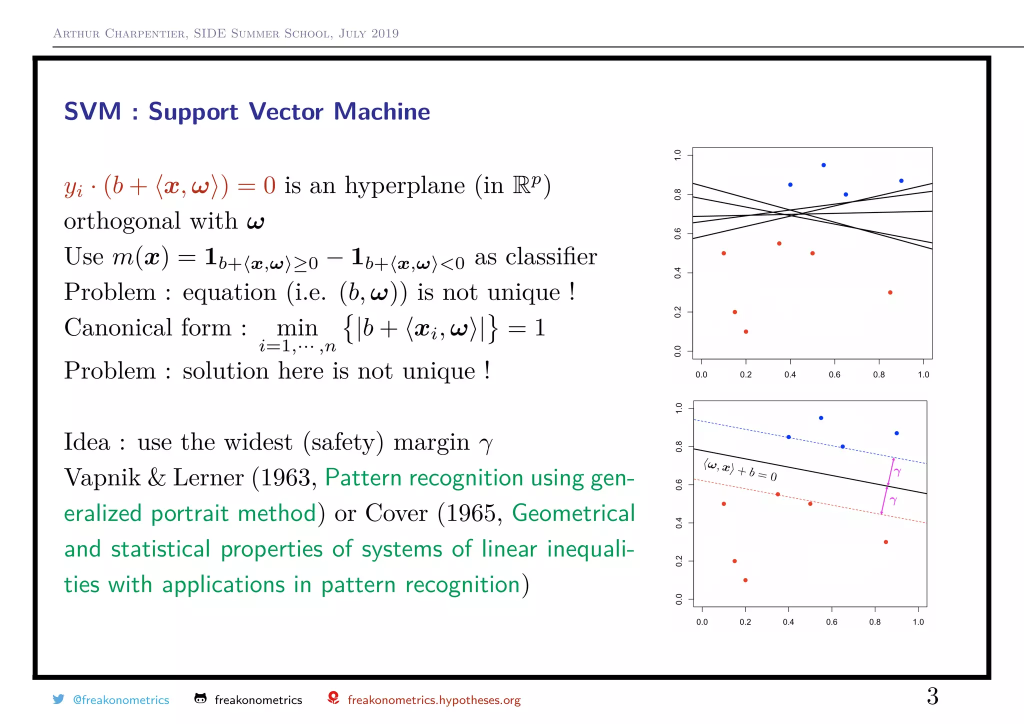
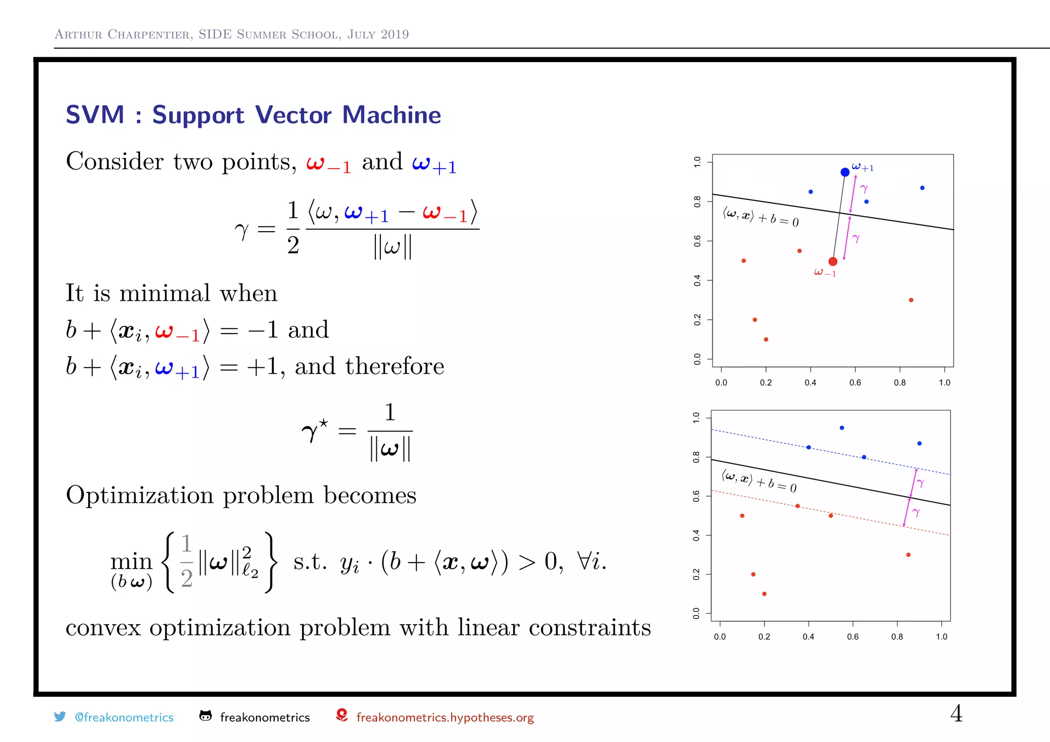
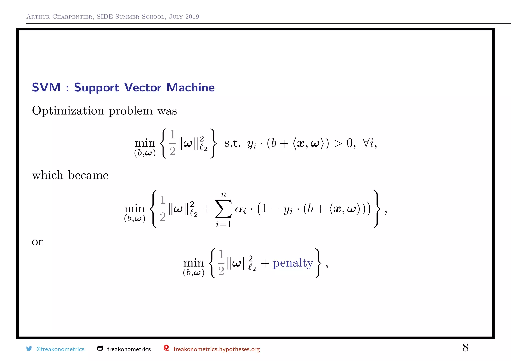
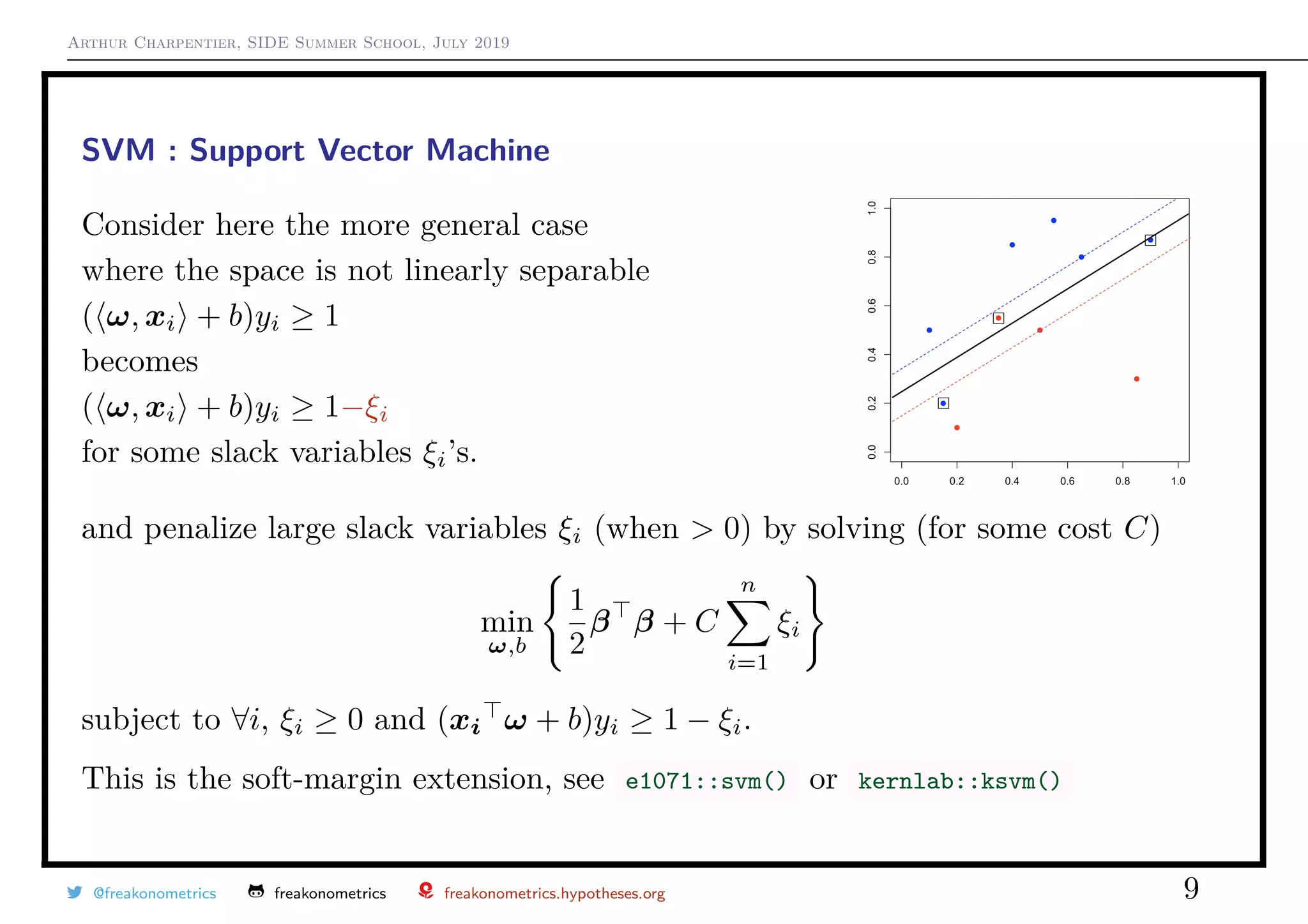
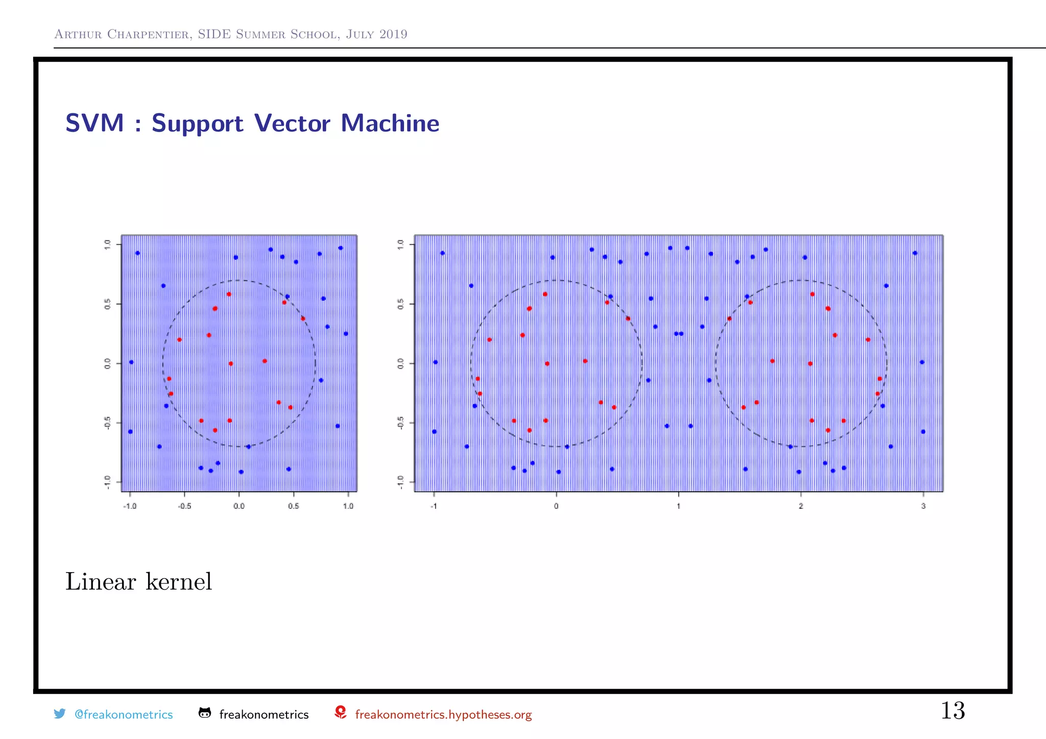
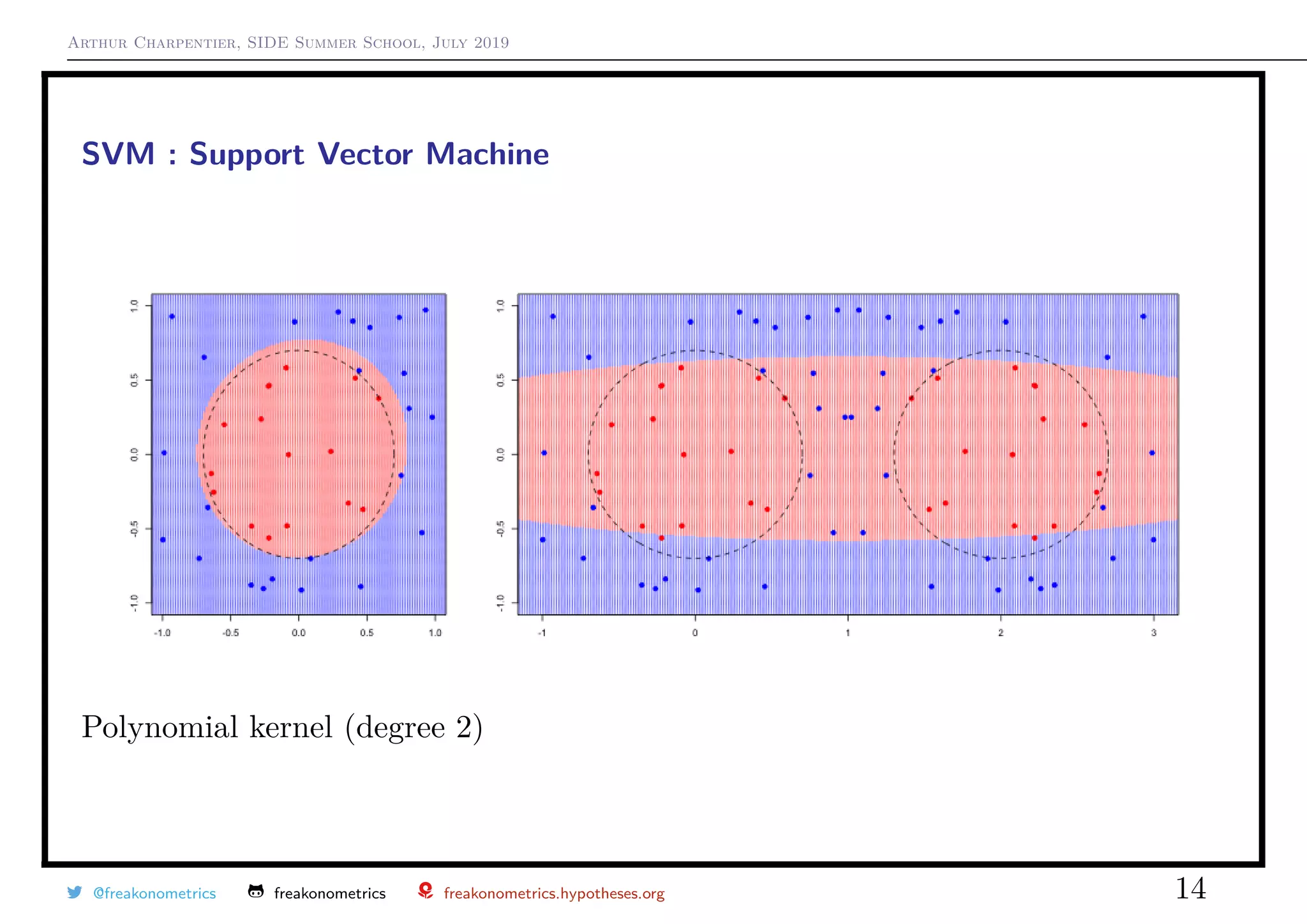
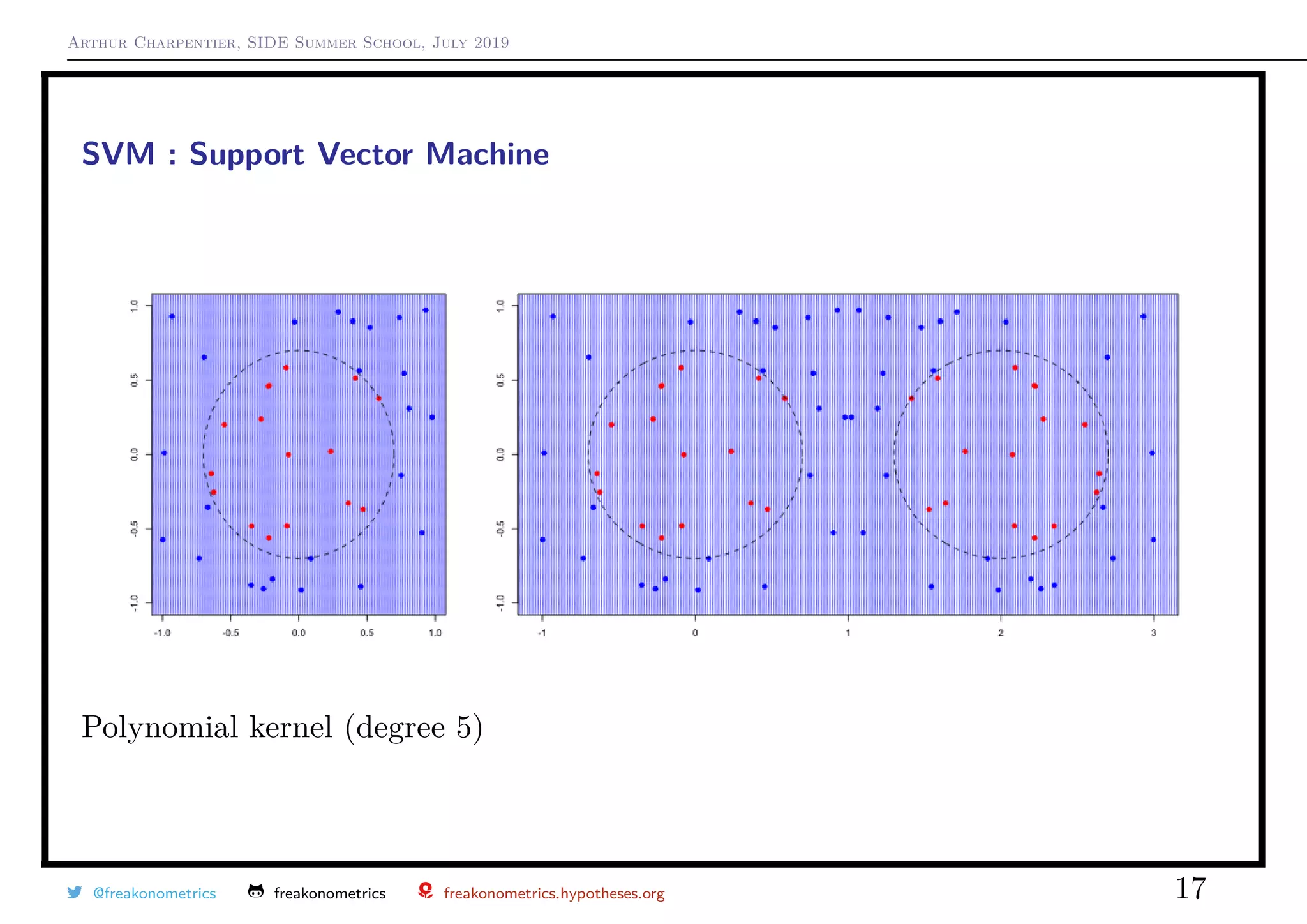
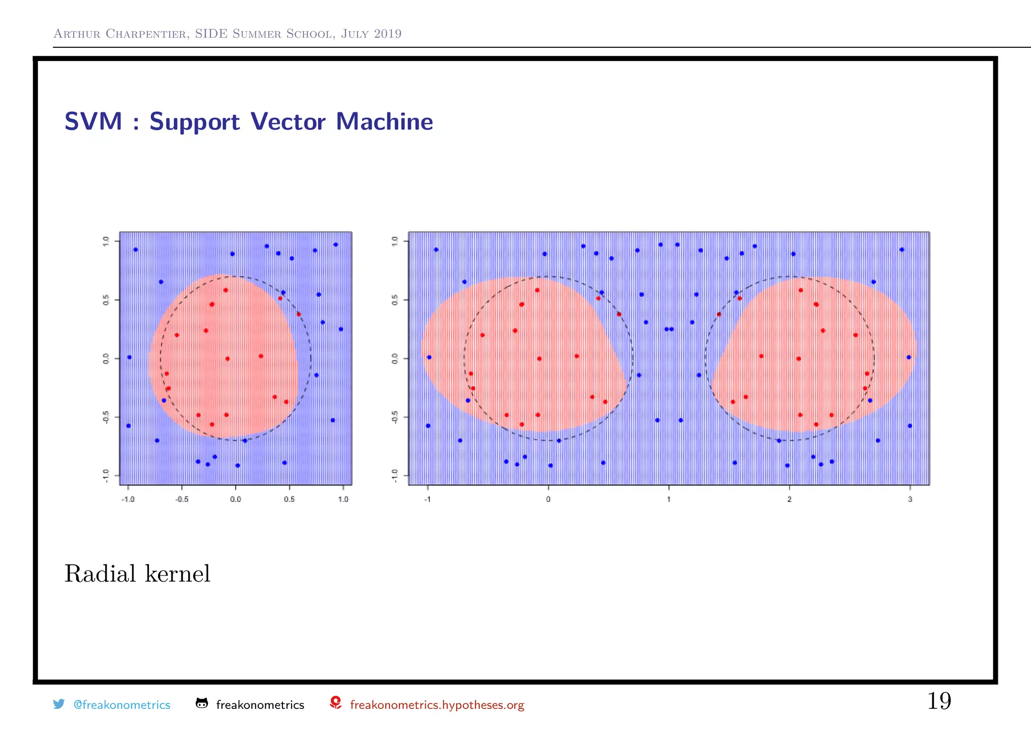
@freakonometrics freakonometrics freakonometrics.hypotheses.org 1

SVM : Support Vector Machine
Linearly Separable sample [econometric notations]
Data (y1, x1), · · · , (yn, xn) - with y ∈ {0, 1} - are
linearly separable if there are (β0, β) such that
- yi = 1 if β0 + x β > 0
- yi = 0 if β0 + x β < 0
Linearly Separable sample [ML notations]
Data (y1, x1), · · · , (yn, xn) - with y ∈ {−1, +1} - are
linearly separable if there are (b, ω) such that
- yi = +1 if b + x, ω > 0
- yi = −1 if b + x, ω < 0
or equivalently yi · (b + x, ω ) > 0, ∀i.

yi · (b + x, ω ) = 0 is an hyperplane (in Rp
)
orthogonal with ω
Use m(x) = 1b+ x,ω ≥0 − 1b+ x,ω <0 as classiﬁer
Problem : equation (i.e. (b, ω)) is not unique !
Canonical form : min
i=1,··· ,n
|b + xi, ω | = 1
Problem : solution here is not unique !
Idea : use the widest (safety) margin γ
Vapnik & Lerner (1963, Pattern recognition using gen-
eralized portrait method) or Cover (1965, Geometrical
and statistical properties of systems of linear inequali-
ties with applications in pattern recognition)

Consider two points, ω−1 and ω+1
γ =
1
2
ω, ω+1 − ω−1
ω
It is minimal when
b + xi, ω−1 = −1 and
b + xi, ω+1 = +1, and therefore
γ =
1
ω
Optimization problem becomes
min
(b ω)
1
2
ω 2
2
s.t. yi · (b + x, ω ) > 0, ∀i.
convex optimization problem with linear constraints

Consider the following problem : min
u∈Rp
h(u) s.t. gi(u) ≥ 0 ∀i = 1, · · · , n
where h is quadratic and gi’s are linear.
Lagrangian is L : Rp
× Rn
→ R deﬁned as L(u, α) = h(u) −
n
i=1
αigi(u)
where α are dual variables, and the dual function is
Λ : α → L(uα, α) = min{L(u, α)} where uα = argmin L(u, α)
One can solve the dual problem, max{Λ(α)} s.t. α ≥ 0. Solution is u = uα .
Si gi(uα ) > 0, then necessarily αi = 0 (see Karush-Kuhn-Tucker (KKT)
condition, αi · gi(uα ) = 0)

Here, L(b, ω, α) =
1
2
ω 2
−
n
i=1
αi · yi · (b + x, ω ) − 1
From the ﬁrst order conditions,
∂L(b, ω, α)
∂ω
= ω −
n
i=1
αi · yixi = 0, i.e. ω =
n
i=1
αi yixi
∂L(b, ω, α)
∂b
= −
n
i=1
αi · yi = 0, i.e.
n
i=1
αi · yi = 0
and
Λ(α) =
n
i=1
αi −
1
2
n
i,j=1
αiαjyiyj αi, αj

min
α
1
2
α Qα − 1 α s.t.



αi ≥ 0, ∀i
y 1 = 0
where Q = [Qi,j] and Qi,j = yiyj xi, xj , and then
ω =
n
i=1
αi yixi and b = −
1
2
min
i:yi=+1
{ xi, ω } + min
i:yi=−1
{ xi, ω }
Points xi such that αi > 0 are called support
yi · (b + xi, ω ) = 1
Use m (x) = 1b + x,ω ≥0−1b + x,ω <0 as classiﬁer
Observe that γ =
n
i=1
α 2
i
−1/2

Optimization problem was
min
(b,ω)
1
2
ω 2
2
s.t. yi · (b + x, ω ) > 0, ∀i,
which became
min
(b,ω)
1
2
ω 2
2
+
n
i=1
αi · 1 − yi · (b + x, ω ) ,
or
min
(b,ω)
1
2
ω 2
2
+ penalty ,

Consider here the more general case
where the space is not linearly separable
( ω, xi + b)yi ≥ 1
becomes
( ω, xi + b)yi ≥ 1−ξi
for some slack variables ξi’s.
and penalize large slack variables ξi (when > 0) by solving (for some cost C)
min
ω,b
1
2
β β + C
n
i=1
ξi
subject to ∀i, ξi ≥ 0 and (xi ω + b)yi ≥ 1 − ξi.
This is the soft-margin extension, see e1071::svm() or kernlab::ksvm()

The dual optimization problem is now
min
α
1
2
α Qα − 1 α s.t.



0 ≤ αi≤ C, ∀i
y 1 = 0
where Q = [Qi,j] and Qi,j = yiyj xi, xj , and then
ω =
n
i=1
αi yixi and b = −
1
2
min
i:yi=+1
{ xi, ω } + min
i:yi=−1
{ xi, ω }
Note further that the (primal) optimization problem can be written
min
(b,ω)
1
2
ω 2
2
+
n
i=1
1 − yi · (b + x, ω ) +
,
where (1 − z)+ is a convex upper bound for empirical error 1z≤0

One can also consider the kernel trick : xi xj is replace by ϕ(xi) ϕ(xj) for some
mapping ϕ,
K(xi, xj) = ϕ(xi) ϕ(xj)
For instance K(a, b) = (a b)3
= ϕ(a) ϕ(b)
where ϕ(a1, a2) = (a3
1 ,
√
3a2
1a2 ,
√
3a1a2
2 , a3
2)
Consider polynomial kernels
K(a, b) = (1 + a b)p
or a Gaussian kernel
K(a, b) = exp(−(a − b) (a − b))
and solve max
αi≥0



n
i=1
αi −
1
2
n
i,j=1
yiyjαiαjK(xi, xj)




Consider the following training sample {(yi, x1,i, x2,i)} with yi ∈ {•, •}

Linear kernel

Polynomial kernel (degree 2)

Radial kernel

SVM : Support Vector Machine - Radial Kernel, impact of the cost C

SVM : Support Vector Machine - Radial Kernel, tuning parameter γ

The radial kernel is formed by taking an inﬁnite sum over polynomial kernels...
K(x, y) = exp − γ x − y 2
= ψ(x), ψ(y)
where ψ is some Rn
→ R∞
function, since
K(x, y) = exp − γ x − y 2
= exp(−γ x 2
− γ y 2
)
=constant
· exp 2γ x, y
i.e.
K(x, y) ∝ exp 2γ x, y =
∞
k=0
2γ
x, y k
k!
=
∞
k=0
2γKk(x, y)
where Kk is the polynomial kernel of degree k.
If K = K1 + K2 with ψj : Rn
→ Rdj
then ψ : Rn
→ Rd
with d ∼ d1 + d2

A kernel is a measure of similarity between vectors.
The smaller the value of γ the narrower the vectors should be to have a small
measure
Is there a probabilistic interpretation ?
Platt (2000, Probabilities for SVM) suggested to use a logistic function over the
SVM scores,
p(x) =
exp[b + x, ω ]
1 + exp[b + x, ω ]

Side 2019 #6

More Related Content

What's hot

Similar to Side 2019 #6

More from Arthur Charpentier

Recently uploaded

Side 2019 #6