The document is a presentation focusing on machine learning, particularly classification using logistic regression and support vector machines (SVMs). It outlines key concepts such as models, inference, and learning, while discussing regularization techniques to prevent overfitting and improving model accuracy. Additionally, it compares logistic regression and SVMs, emphasizing their applications and the importance of selecting appropriate models based on data characteristics.

1. Kriti Puniyani
Carnegie Mellon University
kriti@cmu.edu

2. About me
 Graduate student at Carnegie Mellon University
 Statistical machine learning
 Topic models
 Sparse network learning
 Optimization
 Domains of interest
 Social media analysis
 Systems biology
 Genetics
 Sentiment analysis
 Text processing
4/15/11 2

3. Machine learning
 Computers to “learn with experience”
 Learn : to be able to predict “unseen” things.
 Many applications
 Search
 Machine translation
 Speech recognition
 Vision : identify cars, people, sky, apples
 Robot control
 Introductions :
 http://www.cs.cmu.edu/~tom/pubs/MachineLearning.pdf
 http://videolectures.net/mlss2010_lawrence_mlfcs/
4/15/11 3

4. Classification
 Is this the digit “9” ? ρ
 Will this patient survive ?
 Will this user click on my ad ?
4/15/11 4

5. Predict the next coin toss
Data
Task
THTTTTHHTHTHTTT
Model 1 : Model 2 :
Coin is tossed with Toss depends on wind
probability p (of condition W, starting
being tails) pose S, torque T
Parameters 4/15/11 5

6. Predict the next coin toss
THTTTTHHTHTHTTT
Learning
Model 2 :
Model 1 : W=12.2, S=1,
p=2/3 T=0.23
4/15/11 6

7. Predict the next coin toss
I predict the next
toss to be T
Inference
Model 2 :
Model 1 : W=12.2, S=1,
P=2/3 T=0.23
4/15/11 7

8. Inference
 Parameter : p=2/3
 Predicted next 9 tosses ….H H H T T T T T T
Observed next 9 tosses ….T T T T T T H H H
Accuracy = 2/9 
 Predicted next 9 tosses ….T T T T T T T T T
Observed next 9 tosses ….T T T T T T H H H
Accuracy = 6/9 
 Inference rule :
 if p > 0.5, always predict T,
 if p < 0.5 always predict H. 4/15/11 8

9. The anatomy of classification
1. What is the data (features X, label y) ? ★★★
2. What is the model ? Model parameterization (w)
3. Inference : Given X, w, predict the label.
4. Learning : Given (X,y) pairs, learn the “best” w
 Define “best” – maximize an objective function
(X,Y) pairs train time
Learning
w
test time
(X, ? ) Inference predicted Y
9

10. Logistic Regression
4/15/11 10

11. Predict speaker success
 X = Number of hours spent in preparation
 Y = Was the speaker “good”?
I(a) = 1 if(a==TRUE)
Prediction : Y = I ( X > h) = 0 if(a==FALSE)
4/15/11 11

12. Predict speaker success
Y = I ( X > h)
 Learning is difficult.
 Not robust
4/15/11 12

13. 1
P(Y | w, X) =
1+e−wX +w0
€
Y = I ( X > 10)
4/15/11 13

14. Logistic (sigmoidal) function
4/15/11 14

15. Extend to d dimensions
  1
P(Y | w, X ) = −( w1 X 1 +w 2 X 2 +...+w d X d +w 0 )
1+e
  1
P(Y | w, X ) =  
€ 1+e
−( w. X +w 0 )
4/15/11 15
€

16. Logistic regression
 Model parameter : w
1
P(Y = 1 | w, X) = −wX +w 0
1+e
 Example : Given X = 0.9 , w = 1.2
=> wX = 1.08, P(Y=1|X=0.9) = 0.7465 ~ 0.75
€ Toss a coin with p=3/4
 Example : Given X = -1.1 , w = 1.2
=> wX = -1.32, P(Y=1|X=-1.1) = 0.2108 ~ 0.2
Toss a coin with p=1/5
4/15/11 16

17. Another view of logistic regression
 Log odds : ln [ p/(1-p) ] = wX + ε
 p / (1-p) = ewX
 p = (1-p) ewX
 p (1 + ewX) = ewX
 p = ewX / (1 + ewX) = 1/(e-wX+1)
 Logistic regression is a “linear regression” between log-
odds of an event and features (X)
4/15/11 17

18. The anatomy of classification
1. What is the data (features X, label y) ? ✔
2. What is the model ? Model parameterization (w) ✔
3. Inference :Given X, w, predict the label. ✔
4. Learning : Given (X,y) pairs, learn the “best” w
 Define “best” – maximize an objective function
4/15/11 18

19. Learning : Finding the best w
Expressing…(X , Y )
 Data : (X , Y ),
1 1
Conditional Log Likelihood
n n
 If yi == 1, max P(yi=1| xi, w)
 If yi == 0, max P(yi=0| xi, w)
 Maximize Log-likelihood
4/15/11 19

20. Learning : Example
 Data : (5, 0), (11, 1), (25,1)
l(w)= ln P(y = 0 | x = 5,w) + ln P(y = 1 | x = 11,w) + ln P(y = 1 | x = 25,w)
 P(Y=1|X,w) is a logistic function
1 1
©Carlos Guestrin 2005-2009 1 !
l(w)= ln(1− −5w +w 0
) + ln + ln
1+ e 1+ e−11w +w 0 1+ e−25w +w 0
P(y=1|x) + P(y=0|x) = 1 4/15/11 20
€

21. Optimization : Pick the “best” w
1. Weka
2. Matlab : w = mnrfit(X,Y)
3. R : w <- glm(Y~X, family=binomial(link="logit"))
4. IRLS : http://www.cs.cmu.edu/~ggordon/IRLS-example/logistic.m
5. Implement your own  4/15/11 21

22. Decision surface is linear
Errors
Y=0 Y=1
4/15/11 22

23. Decision surface is linear
http://www.cs.technion.ac.il/~rani/LocBoost/ 4/15/11 23

24. So far..
 Logistic regression is a binary classifier (multinomial
version exists)
 P(Y=1|X,w) is a logistic function
 Inference : Compute P(Y=1|X,w), and do “rounding”.
 Parameter learnt by maximizing log-likelihood of data.
 Decision surface is linear (kernelized version exists)
4/15/11 24

25. Improvements in the model
 Prevent over-fitting Regularization
 Maximize accuracy directly SVMs
 Non-linear decision surface Kernel Trick
 Multi-label data
4/15/11 25

26. Occam’s razor
The simplest explanation is most likely the correct
one
4/15/11 26

27. New and improved learning
 “Best” w == maximize log-likelihood
Maximum Log-likelihood Estimate (MLE)
Small concern … over-fitting
If data is
linearly
separable,
w
4/15/11 27

28. L2 regularization
2
|| w ||2 = ∑ wi
i
2
max w l(w) − λ || w || 2
 Prevents over-fitting
€
 “Pushes” parameters
towards zero
 Equivalent to a prior on
€ the parameters
 Normal distribution (0
mean, unit covariance)
λ : tuning parameter ( 0.1) 4/15/11 28

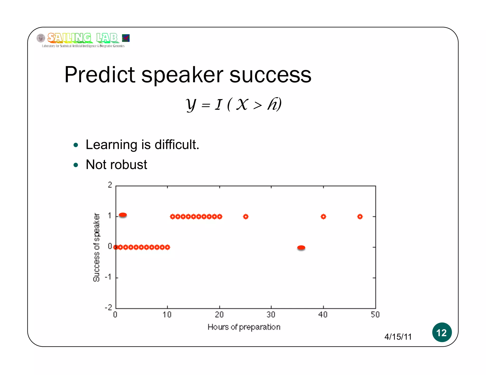
29. Patient Diagnosis
 Y = disease
 X = [age, weight, BP, blood sugar, MRI, genetic tests …]
 Don’t want all “features” to be relevant.
 Weight vector w should be “mostly zeros”.
4/15/11 29

30. L1 regularization || w ||1= ∑ | w i |
i
max w l(w) − λ || w ||1
€
 Prevents over-fitting
 “Pushes” parameters to
zero
 Equivalent to a prior on
€ the parameters
 Laplace distribution
λ increases, more zeros (irrelevant) features 4/15/11 30

31. L1 v/s L2 example
 MLE estimate : [ 11 0.8 ]
 L2 estimate : [ 10 0.6 ] shrinkage
 L1 estimate : [ 10.2 0 ] sparsity
 Mini-conclusion :
 L2 optimization is fast, L1 tends to be slower. If you have the
computational resources, try both (at the same time) !
 ALWAYS run logistic regression with at least some
regularization.
 Corollary : ALWAYS run logistic regression on features that
have been standardized (zero mean, unit variance)
4/15/11 31

32. So far …
 Logistic regression
 Model
 Inference
 Learning via maximum likelihood
 L1 and L2 regularization
Next …. SVMs !
4/15/11 32

33. Why did we use probability again?
 Aim : Maximize “accuracy”
 Logistic regression : Indirect method that maximizes
likelihood of data.
 A much more direct approach is to directly maximize
accuracy.
Support Vector Machines (SVMs)
4/15/11 33

34. Maximize the margin
Maximize the margin
! 2005-2007 Carlos Guestrin "
4/15/11 34

35. Geometry review
Y=1 2x1+x2-2=0
Y= -1
For a point on the line :
(0.5, 1 ) : d = 2*0.5 + 1 – 2 =0
Signed “distance” to the line from (x10, x20)
d = 2x10 + x20 - 2 4/15/11 35

36. Geometry review
Y=1 2x1+x2-2=0
Y= -1
(1, 2.5) : d = 2*1 + 2.5 - 2 = 2.5 > 0
y(wx+b) = 1*2.5 = 2.5 > γ
4/15/11 36

37. Geometry review
Y=1 2x1+x2-2=0
Y= -1
(0.5, 0.5) : d = 2*0.5 + 0.5 – 2 = -0.5 < 0
y(w.x+b) = y*d = -1 * -0.5 = 0.5
4/15/11 37

38. Support Vector Machines
Normalized margin – Canonical
hyperplanes
! 2005-2007 Carlos Guestrin "
Support vectors are the
x+ points touching the margins.
x-
4/15/11 38
! 2005-2007 Carlos Guestrin !

39. = !j w(j) x(j)
! 2005-2007 Carlos Guestrin !
w.x = !j w(j) x(j)
w.x = !j w(j) x(j)
! 2005-2007 Carlos Guestrin !
Slack variables ! 2005-2007 Carlos Guestrin
 SVMs are made robust by adding “slack variables” that
allow training error to be non-zero
ximize the margin point. Slack variable ==0 for correctly
 One for each data
Maximizepoints. margin
classified the
Maximize the−C∑ξ i
max γ margin
€
4/15/11 39

40. Slack variables
max γ −C ∑ξ i
€
Need to tune C :
high C == minimize mis-classifications
low C == maximize margin
4/15/11 40

41. SVM summary
 Model : w.x + b > 0 if y = +1
w.x + b < 0 if y = -1
 Inference : ŷ = sign(w.x+b)
 Learning : Maximize { (margin) - C ( slack-variables) }
Next … Kernel SVMs
4/15/11 41

42. The kernel trick
 Why linear separator ? What if data looks like below ?
The kernel trick
allows you to use
SVMs with non-
linear separators.
Different kernels
1. Polynomial
2. Gaussian
3. exponential
4/15/11 42

43. Logistic Linear SVM
Error ~ 40% in both cases
4/15/11 43

44. Kernel SVM with polynomial kernel
of degree 2
Polynomial kernel of
degree 2/4 do very
well, but degree 3/5
do very bad.
Gaussian kernel has
tuning parameter
(bandwidth).
Performance
depends on picking
the right bandwith.
Error = 7% 4/15/11 44

45. SVMs summary
 Maximize the margin between positive and negative
examples.
 Kernel trick is widely implemented, allowing non-linear
decision surface.
 Not probabilistic 
 Software :
 SVM-light http://svmlight.joachims.org/,
 LIBSVM http://www.csie.ntu.edu.tw/~cjlin/libsvm/
 Weka, matlab, R
4/15/11 45

46. Demo
http://www.cs.technion.ac.il/~rani/LocBoost
4/15/11 46

47. Which to use ?
 Linear SVMs and logistic regression work very similar in
most cases.
 Kernelized SVMs work better than linear SVMs (mostly)
 Kernelized logistic regression is possible, but
implementations are not available easily.
4/15/11 47

48. Recommendations
1. First, try logistic regression. Easy, fast, stable. No “tuning”
parameters.
2. Equivalently, you can first try linear SVMs, but you need
to tune “C”
3. If results are “good enough”, stop.
4. Else try SVMs with Gaussian kernels.
Need to tune bandwidth, C – by using validation data.
If you have more time/computational resources, try random
forests as well.
** Recommendations are opinions of the presenter, and not known facts.
4/15/11 48

49. In conclusion …
 Logistic Regression
 Support Vector Machines
Other classification approaches …
 Random forests / decision trees
 Naïve Bayes
 Nearest Neighbors
 Boosting (Adaboost)
4/15/11 49

50. Thank you
Questions?
4/15/11 50

51. Kriti Puniyani
Carnegie Mellon University
kriti@cmu.edu

52. Is this athlete doing drugs ?
 X = Blood-test-to-detect-drugs
 Y = Doped athlete ?
 Two types of errors :
 Athlete is doped, we predict “NO” : false negative
 Athlete is NOT doped, we predict “YES” : false positive
 Penalize false positives more than false negatives
4/15/11 52

53. Outline
 What is classification ?
 Parameters, data, inference, learning
 Predicting coin tosses (0-dimensional X)
 Logistic Regression
 Predicting “speaker success” (1-dimensional X)
 Formulation, optimizatiob
 Decision surface is linear
 Interpreting coefficients
 Hypothesis testing
 Evaluating the performance of the model
 Why is it called “regression” : log-odds
 L2 regularization
 Patient survival (d-dimensional X)
 L1 regularization
 Support Vector Machines
 Linear SVMs + formulation
 What are “support vectors”
 The kernel trick
 Demo : logistic regression v/s SVMs v/s kernel tricks 4/15/11 53

54. Overfitting a more serious problem
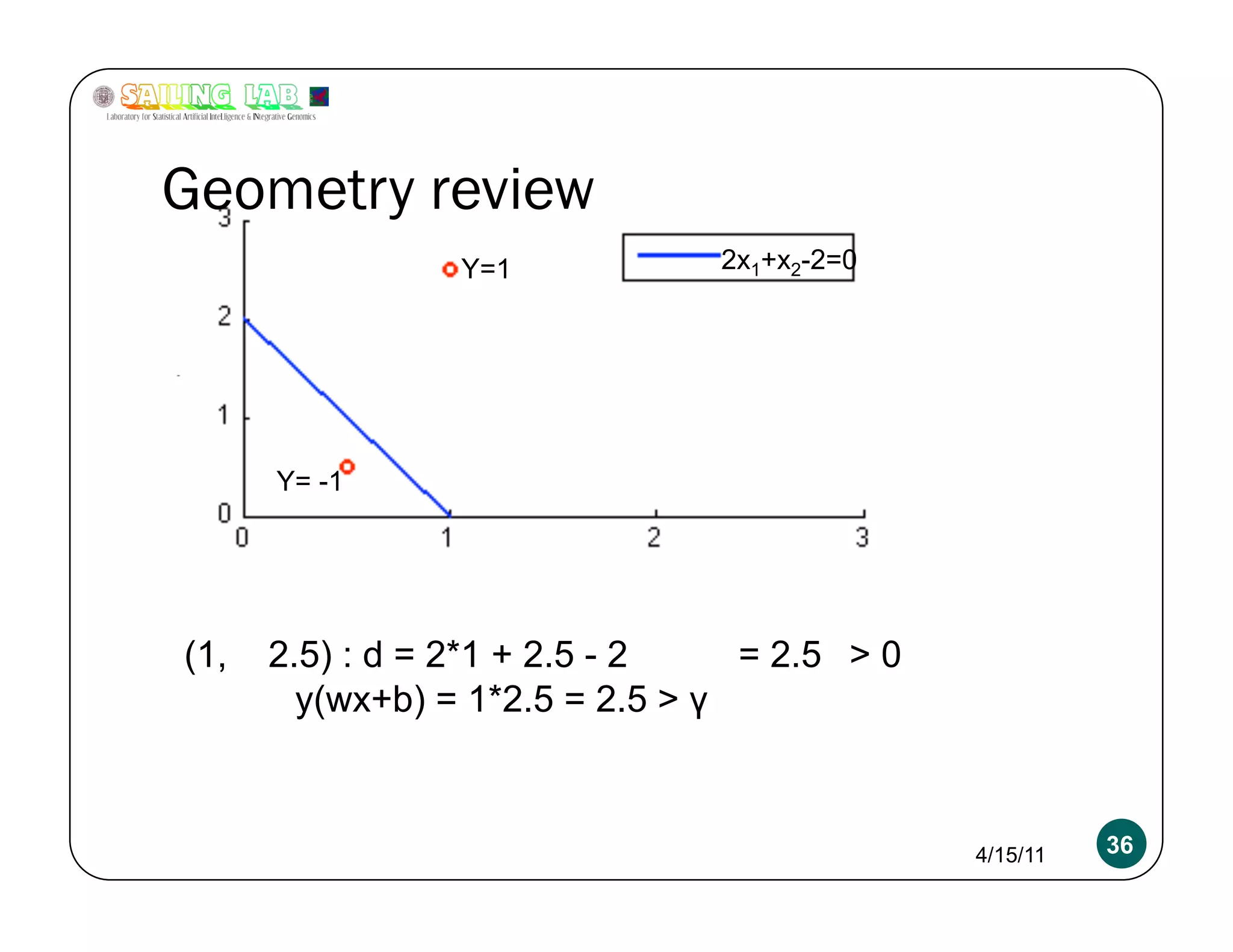
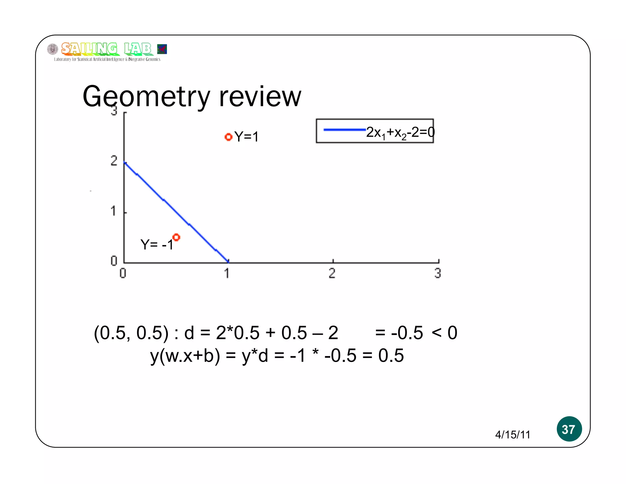
2x+y-2 = 0 w = [2 1 -2]
4x+2y-4 = 0 w = [4 2 -4]
400x+200y-400 = 0 w = [400 200 -400]
 Absolutely need L2 regularization 4/15/11 54