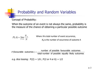
The document provides an overview of probability theory and random variables including: 1) It defines probability as a measure of the chance of obtaining a particular outcome from an event. Common properties of probability such as mutually exclusive events and conditional probability are also covered. 2) Random variables are introduced as rules that assign real numbers to possible outcomes of an experiment. Both discrete and continuous random variables are defined. 3) Key concepts related to random variables are summarized including the cumulative distribution function, probability density function, expected value, variance, and common distributions like the uniform, binomial, and Gaussian distributions. 4) Finally, random processes are defined as sets of random variables indexed by time, with properties like the mean

1. TELE3113 Analogue & Digital
Communications
Review of Probability Theory
p. 1

2. Probability and Random Variables
Concept of Probability:
When the outcome of an event is not always the same, probability is
the measure of the chance of obtaining a particular possible outcome
NA Where N is total number of event occurrence,
P( A) = lim
N →∞ N
NA is the number of occurrence of outcome A
number of possible favourable outcomes
P ( favourable outcomes ) =
total number of possible equally likely outcomes
e.g. dice tossing: P{2} = 1/6 ; P{2 or 4 or 6} = 1/2
p. 2

3. Common Properties of Probability
• 0≤ P(A) ≤ 1 N
• If there are N possible outcomes {A1 , A2 , … , AN} then ∑ P( A ) = 1
i =1
i
• Conditional Probability:
probability of the outcome of an event is conditional on the outcome of
another event
P(A and B) P(A and B)
P(B | A) =
P(A)
; P(A | B) =
P(B)
P( A) P(B | A)
Bayes’ theorem P(A | B) =
P(B)
p. 3

4. Common Properties of Probability
• Mutually exclusiveness
P(A or B) = P(A) + P(B); P(A and B) = 0
Thus, A and B are mutually exclusive.
• Statistically Independence
P(B | A) = P( B ) ; P(A | B) = P( A)
⇒ P(A and B) = P(A) ⋅ P(B) Q P(B | A) =
P(A and B)
P(A)
; P(A | B) =
P(A and B)
P(B)
Thus, A and B are statistically independent.
p. 4

5. Communication Example
In a communication channel, signal may be corrupted by noises.
P(r0|m0)
m0 r0
P(r0|m1)
P(r1|m0)
m1 r1
P(r1|m1)
If r0 is received, m0 should be chosen if
P(m0|r0)P(r0) > P(m1|r0)P(r0)
By Bayes’ theorem P(r0|m0)P(m0) > P(r0|m1)P(m1)
Similarly, if r1 is received, m1 should be chosen if
P(m1|r1)P(r1) > P(m0|r1)P(r1) ⇒ P(r1|m1)P(m1) > P(r1|m0)P(m0)
Probability of correct reception: P(c) = P(ro|mo)P(mo) + P(r1|m1)P(m1)
Probability of error: P(ε) = 1-P(c)
p. 5

6. Random Variables
A random variable X(.) is the rule or functional relationship which assigns
real numbers X(λi) to each possible outcome λi in an experiment.
For example, in coin tossing, we can assign X(head) = 1, X(tail) = -1
If X(λ) assumes a finite number of distinct values
discrete random variable
If X(λ) assumes any values within an interval
continuous random variable
p. 6

7. Cumulative Distribution Function
The cumulative distribution function, FX(x) , associated with a random
variable X is: FX(x)
FX ( x) = P{ X ≤ x} 1
Properties:
• 0 ≤ FX ( x ) ≤ 1
• F (−∞) = 0; F (∞) = 1
0 x
• F ( x1 ) ≤ F ( x 2 ) if x1 ≤ x 2 (Non-decreasing)
FX(x)
•
P{x1 < X ≤ x 2 } = FX ( x 2 ) − FX ( x1 ) 1
0 x
p. 7

8. Probability Density Function
The probability density function, fX(x) , associated with a random variable
X is: dF ( x)
f X ( x) = X FX(x)
dx
Properties: 1
• f X ( x) ≥ 0 for all x
∞
0 x
• ∫f
−∞
X ( x)dx = 1
fX(x)
x
• P{ X ≤ x} = FX ( x) = ∫f
−∞
X ( β )dβ
x2
• P{x1 < X ≤ x 2 } = FX ( x 2 ) − FX ( x1 ) = ∫f
x1
X ( x)dx
0 x
p. 8

9. Statistical Averages of Random Variables
The statistical average or expected value of a random variable X is
∞
defined as
E{ X } =∑i
∫
xi P ( xi ) = m X or E{ X } = xf ( x)dx = m X
−∞
E{X} is called the first moment of X and mX is the average or mean
value of X.
Similarly, the second moment E{X2} is ∞
E{ X 2 } = ∑ xi P ( xi ) E{ X 2 } = ∫ x 2 f ( x)dx
2
or
i −∞
Its square root is called the root-mean-square (rms) value of X.
The variance of the random variable X is defined as
∞
σ X = E{( X − m X ) 2 } = ∫ ( X − m X ) 2 f ( x)dx or σ X 2 = E{ X 2 } − m X 2
2
−∞
The square root of the variance is called the standard deviation, σX, of the
random variable X.
p. 9

10. Statistical Averages of Random Variables
Expected value of linear combination of N random variables is
equivalent to linear combination of expected values of individual
random variables N  N
E ∑ ai X i  = ∑ ai E{ X i }
 i =1  i =1
For N statistically independent random variables: X1, X2, … , XN
N  N 2
Var ∑ ai X i  = ∑ ai Var{ X i }
 i =1  i =1
Covariance of a pair of random variables: X, Y
µ XY = E{( X − m X )(Y − mY )} = E{ XY } − m X mY
If X and Y are statistically independent, µXY=0
p. 10

11. Uniform Distribution
A random variable that is equally likely to take on any value within a
given range is said to be uniformly distributed.
p. 11

12. Binomial Distribution
Consider an experiment having only two possible outcomes, A and B,
which are mutually exclusive.
Let the probabilities be P(A) = p and P(B) = 1 − p = q.
The experiment is repeated n times and the probability of A occurring i
times is P ( A = i ) =  n  p i q n − i , where  n  =
   
n!
(binomial coefficient).
   
i! ( n − i )!
i i
The mean value of the binomial distribution is np and the variance is (npq).
p. 12

13. Gaussian Distribution
Central-Limit theorem: The sum of N independent, identically distributed
random variables approaches a Gaussian distribution
when N is very large.
The Gaussian pdf is continuous and is defined by
1 − ( x − µ ) 2 / 2σ 2
f ( x) = e
2π σ
where µ is the mean ,
and σ2 is the variance .
cumulative distribution function:
FX ( x) = P{ X ≤ x}
x
1
∫
− ( y − µ ) 2 / 2σ 2
= e dy
−∞ 2π σ
p. 13

14. Gaussian Distribution
1 − x2 / 2
Zero-mean unit-variance Gaussian random variable: g ( x) = 2π e
x x
1
∫ g ( y)dy = ∫
2
⇒ Probability distribution function: Ω( x) = e−y /2
dy
−∞ 2π −∞
∞
1
∫e
− y2 / 2
Define Q-function: Q( x) = 1 − Ω( x) = dy (monotonic decreasing)
2π x
1 − ( x − µ ) 2 / 2σ 2
In general, for a random variable X with pdf: f ( x) = e
2π σ
x−µ x−µ
P ( X ≤ x) = Ω  ; P ( X > x ) = Q 
 σ   σ 
Define: error function (erf) and complementary error function (erfc) :
x ∞
2 2
∫e ∫e
2
−y − y2
erf ( x) = dy ; erfc( x) = 1 − erf ( x) = dy
π 0 π x
Thus,
1  x  1  x 
Ω( x) = 1 + erf   ; Q(x) = erfc 
2  2  2  2
p. 14

15. Q-function
∞
1
∫
2
Q ( x) = e−y /2
dy
2π x
2
e−x /2
Q ( x) ≅ for x >> 1
x 2π
p. 15

16. Random Processes
A random process is a set of indexed random variables (sample functions)
defined in the same probability space.
In communications, the index is usually in terms of time.
xi(t) is called a sample function
of the sample space.
The set of all possible sample functions
{xi(t)} is called ensemble and defines
the random process X(t).
For a specific i, xi(t) is a time function.
For a specific ti, X(ti) denotes a random
variable.
p. 16

17. Random Processes: Properties
Consider a random process X(t) , let X(tk) denote the random variable
obtained by observing the process X(t) at time tk .
Mean: mX(tk) =E{X(tk)}
Variance:σX2 (tk) =E{X2(tk)}-[mX (tk)] 2
Autocorrelation: RX{tk ,tj}=E{X(tk)X(tj)} for any tk and tj
Autocovariance: CX{tk ,tj}=E{ [X(tk)- mX (tk)][X(tj)- mX (tj)] }
p. 17