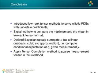
The document discusses tensor completion for partial differential equations (PDEs) with uncertain coefficients and Bayesian updates, emphasizing the importance of uncertainty quantification in simulations. It covers the stochastic forward problem, Bayesian updating methods, including Gaussian filters, and describes a tensor completion approach to handle these uncertainties efficiently. The document provides examples and techniques related to discretization, polynomial chaos expansions, and conditional expectations in the context of PDEs.

1. Tensor completion for PDEs with uncertain
coefficients and Bayesian Update
Alexander Litvinenko
(joint work with E. Zander, B. Rosic, O. Pajonk, H. Matthies)
Center for Uncertainty
Quantification
ntification Logo Lock-up
http://sri-uq.kaust.edu.sa/
Extreme Computing Research Center, KAUST
Alexander Litvinenko (joint work with E. Zander, B. Rosic, O. Pajonk, H. Matthies)Tensor completion for PDEs with uncertain coefficients and B

2. 4*
The structure of the talk
Part I (Stochastic forward problem):
1. Motivation
2. Elliptic PDE with uncertain coefficients
3. Discretization and low-rank tensor approximations
Part II (Bayesian update):
1. Bayesian update surrogate
2. Examples
Part III (Tensor completion):
1. Problem setup
2. Tensor completion for Bayesian Update

3. 4*
Motivation to do Uncertainty Quantification (UQ)
Motivation: there is an urgent need to quantify and reduce the
uncertainty in output quantities of computer simulations within
complex (multiscale-multiphysics) applications.
Typical challenges: classical sampling methods are often very
inefficient, whereas straightforward functional representations
are subject to the well-known Curse of Dimensionality.
Nowadays computational predictions are used in critical
engineering decisions and thanks to modern computers we are
able to simulate very complex phenomena. But, how reliable
are these predictions? Can they be trusted?
Example: Saudi Aramco currently has a simulator,
GigaPOWERS, which runs with 9 billion cells. How sensitive
are the simulation results with respect to the unknown reservoir
properties?
Center for Uncertainty
Quantification
ation Logo Lock-up
3 / 30

4. 4*
Part I: Stochastic forward problem
Part I: Stochastic Galerkin method to solve
elliptic PDE with uncertain coefficients

5. 4*
PDE with uncertain coefficient and RHS
Consider
− div(κ(x, ω) u(x, ω)) = f(x, ω) in G × Ω, G ⊂ R2,
u = 0 on ∂G,
(1)
where κ(x, ω) - uncertain diffusion coefficient. Since κ positive,
usually κ(x, ω) = eγ(x,ω).
For well-posedness see [Sarkis 09, Gittelson 10, H.J.Starkloff
11, Ullmann 10].
Further we will assume that covκ(x, y) is given.
Center for Uncertainty
Quantification
ation Logo Lock-up
4 / 30

6. 4*
My previous work
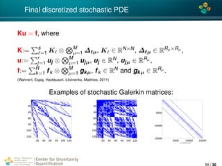
After applying the stochastic Galerkin method, obtain:
Ku = f, where all ingredients are represented in a tensor format
Compute max{u}, var(u), level sets of u, sign(u)
[1] Efficient Analysis of High Dimensional Data in Tensor Formats,
Espig, Hackbusch, A.L., Matthies and Zander, 2012.
Research which ingredients influence on the tensor rank of K
[2] Efficient low-rank approximation of the stochastic Galerkin matrix in tensor formats,
W¨ahnert, Espig, Hackbusch, A.L., Matthies, 2013.
Approximate κ(x, ω), stochastic Galerkin operator K in Tensor
Train (TT) format, solve for u, postprocessing
[3] Polynomial Chaos Expansion of random coefficients and the solution of stochastic
partial differential equations in the Tensor Train format, Dolgov, Litvinenko, Khoromskij, Matthies, 2016.
Center for Uncertainty
Quantification
ation Logo Lock-up
5 / 30

7. 4*
Canonical and Tucker tensor formats
Definition and Examples of tensors
Center for Uncertainty
Quantification
ation Logo Lock-up
6 / 30

8. 4*
Canonical and Tucker tensor formats
[Pictures are taken from B. Khoromskij and A. Auer lecture course]
Storage: O(nd ) → O(dRn) and O(Rd + dRn).
Center for Uncertainty
Quantification
ation Logo Lock-up
7 / 30

9. 4*
Definition of tensor of order d
Tensor of order d is a multidimensional array over a d-tuple
index set I = I1 × · · · × Id ,
A = [ai1...id
: iµ ∈ Iµ] ∈ RI
, Iµ = {1, ..., nµ}, µ = 1, .., d.
A is an element of the linear space
Vn =
d
µ=1
Vµ, Vµ = RIµ
equipped with the Euclidean scalar product ·, · : Vn × Vn → R,
defined as
A, B :=
(i1...id )∈I
ai1...id
bi1...id
, for A, B ∈ Vn.
Center for Uncertainty
Quantification
ation Logo Lock-up
8 / 30

10. 4*
Discretization of elliptic PDE
Now let us discretize our diffusion equation with
uncertain coefficients
Center for Uncertainty
Quantification
ation Logo Lock-up
9 / 30

11. 4*
Karhunen Lo´eve and Polynomial Chaos Expansions
Apply both
Karhunen Lo´eve Expansion (KLE):
κ(x, ω) = κ0(x) + ∞
j=1 κjgj(x)ξj(θ(ω)), where
θ = θ(ω) = (θ1(ω), θ2(ω), ..., ),
ξj(θ) = 1
κj G (κ(x, ω) − κ0(x)) gj(x)dx.
Polynomial Chaos Expansion (PCE)
κ(x, ω) = α κ(α)(x)Hα(θ), compute ξj(θ) = α∈J ξ
(α)
j Hα(θ),
where ξ
(α)
j = 1
κj G κ(α)(x)gj(x)dx.
Further compute ξ
(α)
j ≈ s
=1(ξ )j
∞
k=1(ξ , k )αk
.
Center for Uncertainty
Quantification
ation Logo Lock-up
10 / 30

12. 4*
Final discretized stochastic PDE
Ku = f, where
K:= s
=1 K ⊗ M
µ=1 ∆ µ, K ∈ RN×N, ∆ µ ∈ RRµ×Rµ ,
u:= r
j=1 uj ⊗ M
µ=1 ujµ, uj ∈ RN, ujµ ∈ RRµ ,
f:= R
k=1 fk ⊗ M
µ=1 gkµ, fk ∈ RN and gkµ ∈ RRµ .
(Wahnert, Espig, Hackbusch, Litvinenko, Matthies, 2011)
Examples of stochastic Galerkin matrices:
Center for Uncertainty
Quantification
ation Logo Lock-up
11 / 30

13. 4*
Part II
Part II: Bayesian update
We will speak about Gauss-Markov-Kalman filter for the
Bayesian updating of parameters in comput. model.

14. 4*
Mathematical setup
Consider
K(u; q) = f ⇒ u = S(f; q),
where S is solution operator.
Operator depends on parameters q ∈ Q,
hence state u ∈ U is also function of q:
Measurement operator Y with values in Y:
y = Y(q; u) = Y(q, S(f; q)).
Examples of measurements:
y(ω) = D0
u(ω, x)dx, or u in few points
Center for Uncertainty
Quantification
ation Logo Lock-up
12 / 30

15. 4*
Random QoI
With state u a RV, the quantity to be measured
y(ω) = Y(q(ω), u(ω)))
is also uncertain, a random variable.
Noisy data: ˆy + (ω),
where ˆy is the “true” value and a random error .
Forecast of the measurement: z(ω) = y(ω) + (ω).
Center for Uncertainty
Quantification
ation Logo Lock-up
13 / 30

16. 4*
Conditional probability and expectation
Classically, Bayes’s theorem gives conditional probability
P(Iq|Mz) =
P(Mz|Iq)
P(Mz)
P(Iq) (or πq(q|z) =
p(z|q)
Zs
pq(q));
Expectation with this posterior measure is conditional
expectation.
Kolmogorov starts from conditional expectation E (·|Mz),
from this conditional probability via P(Iq|Mz) = E χIq
|Mz .
Center for Uncertainty
Quantification
ation Logo Lock-up
14 / 30

17. 4*
Conditional expectation
The conditional expectation is defined as
orthogonal projection onto the closed subspace L2(Ω, P, σ(z)):
E(q|σ(z)) := PQ∞ q = argmin˜q∈L2(Ω,P,σ(z)) q − ˜q 2
L2
The subspace Q∞ := L2(Ω, P, σ(z)) represents the available
information.
The update, also called the assimilated value
qa(ω) := PQ∞ q = E(q|σ(z)), is a Q-valued RV
and represents new state of knowledge after the measurement.
Doob-Dynkin: Q∞ = {ϕ ∈ Q : ϕ = φ ◦ z, φ measurable}.
Center for Uncertainty
Quantification
ation Logo Lock-up
15 / 30

18. 4*
Numerical computation of NLBU
Look for ϕ such that q(ξ) = ϕ(z(ξ)), z(ξ) = y(ξ) + ε(ω):
ϕ ≈ ˜ϕ =
α∈Jp
ϕαΦα(z(ξ))
and minimize q(ξ) − ˜ϕ(z(ξ)) 2
L2
, where Φα are polynomials
(e.g. Hermite, Laguerre, Chebyshev or something else).
Taking derivatives with respect to ϕα:
∂
∂ϕα
q(ξ) − ˜ϕ(z(ξ)), q(ξ) − ˜ϕ(z(ξ)) = 0 ∀α ∈ Jp
Inserting representation for ˜ϕ, obtain:
Center for Uncertainty
Quantification
ation Logo Lock-up
16 / 30

19. 4*
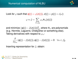
Numerical computation of NLBU
∂
∂ϕα
E

q2
(ξ) − 2
β∈J
qϕβΦβ(z) +
β,γ∈J
ϕβϕγΦβ(z)Φγ(z)


= 2E

−qΦα(z) +
β∈J
ϕβΦβ(z)Φα(z)


= 2


β∈J
E [Φβ(z)Φα(z)] ϕβ − E [qΦα(z)]

 = 0 ∀α ∈ J .
Center for Uncertainty
Quantification
ation Logo Lock-up
17 / 30

20. 4*
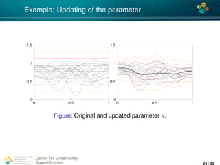
Numerical computation of NLBU
Now, rewriting the last sum in a matrix form, obtain the linear
system of equations (=: A) to compute coefficients ϕβ:



... ... ...
... E [Φα(z(ξ))Φβ(z(ξ))]
...
... ... ...







...
ϕβ
...



 =




...
E [q(ξ)Φα(z(ξ))]
...



 ,
where α, β ∈ J , A is of size |J | × |J |.
Center for Uncertainty
Quantification
ation Logo Lock-up
18 / 30

21. 4*
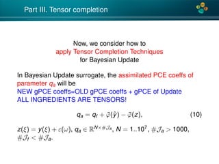
Numerical computation of NLBU
We can rewrite the system above in the compact form:
[Φ] [diag(...wi...)] [Φ]T




...
ϕβ
...



 = [Φ]


w0q(ξ0)
...
wNq(ξN)


[Φ] ∈ RJα×N, [diag(...wi...)] ∈ RN×N, [Φ] ∈ RJα×N.
Solving this system, obtain vector of coefficients (...ϕβ...)T for
all β.
Finally, the assimilated parameter qa will be
qa = qf + ˜ϕ(ˆy) − ˜ϕ(z), (2)
z(ξ) = y(ξ) + ε(ω), ˜ϕ = β∈Jp
ϕβΦβ(z(ξ))
Center for Uncertainty
Quantification
ation Logo Lock-up
19 / 30

22. 4*
Explanation of ” Bayesian Update surrogate” from E. Zander
Let the stochastic model of the measurement is given by
y = M(q) + ε, ε -measurement noise (3)
Best estimator ˜ϕ for q given z, i.e.
˜ϕ = argminϕ E[ q(·) − ϕ(z(·)) 2
2]. (4)
The best estimate (or predictor) of q given the
measurement model is
qM(ξ) = ˜ϕ(z(ξ))). (5)
The remainder, i.e. the difference between q and qM, is
given by
q⊥
M(ξ) = q(ξ) − qM(ξ), (6)
Due to the minimisation property of the MMSE
estimator—orthogonal to qM(ξ), i.e. cov(q⊥
M, qM) = 0.
Center for Uncertainty
Quantification
ation Logo Lock-up
20 / 30

23. In other words,
q(ξ) = qM(ξ) + q⊥
M(ξ) (7)
yields an orthogonal decomposition of q.
Actual measurement ˆy, prediction ˆq = ˜ϕ(ˆy). Part qM of q
can be “collapsed” to ˆq. Updated stochastic model q is
thus given by
q (ξ) = ˆq + q⊥
M(ξ) (8)
q (ξ) = q(ξ) + ( ˜ϕ(ˆy) − ˜ϕ(z(ξ))). (9)
Center for Uncertainty
Quantification
ation Logo Lock-up
21 / 30

24. 4*
Example: 1D elliptic PDE with uncertain coeffs
− · (κ(x, ξ) u(x, ξ)) = f(x, ξ), x ∈ [0, 1]
+ Dirichlet random b.c. g(0, ξ) and g(1, ξ).
3 measurements: u(0.3) = 22, s.d. 0.2, x(0.5) = 28, s.d. 0.3,
x(0.8) = 18, s.d. 0.3.
κ(x, ξ): N = 100 dofs, M = 5, number of KLE terms 35, beta distribution for κ, Gaussian covκ, cov.
length 0.1, multi-variate Hermite polynomial of order pκ = 2;
RHS f(x, ξ): Mf = 5, number of KLE terms 40, beta distribution for κ, exponential covf , cov. length 0.03,
multi-variate Hermite polynomial of order pf = 2;
b.c. g(x, ξ): Mg = 2, number of KLE terms 2, normal distribution for g, Gaussian covg , cov. length 10,
multi-variate Hermite polynomial of order pg = 1;
pφ = 3 and pu = 3
Center for Uncertainty
Quantification
ation Logo Lock-up
22 / 30

25. 4*
Example: updating of the solution u
0 0.5 1
-20
0
20
40
60
0 0.5 1
-20
0
20
40
60
Figure: Original and updated solutions, mean value plus/minus 1,2,3
standard deviations
[graphics are built in the stochastic Galerkin library sglib, written by E. Zander in TU Braunschweig]
Center for Uncertainty
Quantification
ation Logo Lock-up
23 / 30

26. 4*
Example: Updating of the parameter
0 0.5 1
0
0.5
1
1.5
0 0.5 1
0
0.5
1
1.5
Figure: Original and updated parameter κ.
Center for Uncertainty
Quantification
ation Logo Lock-up
24 / 30

27. 4*
Part III. Tensor completion
Now, we consider how to
apply Tensor Completion Techniques
for Bayesian Update
In Bayesian Update surrogate, the assimilated PCE coeffs of
parameter qa will be
NEW gPCE coeffs=OLD gPCE coeffs + gPCE of Update
ALL INGREDIENTS ARE TENSORS!
qa = qf + ˜ϕ(ˆy) − ˜ϕ(z), (10)
z(ξ) = y(ξ) + ε(ω), qa ∈ RN×#Ja , N = 1..107, #Ja > 1000,
#Jf < #Ja.

28. 4*
Problem setup: Tensor completion
Problem of fitting a low rank tensor A ∈ RI, I := I1 × ... × Id ,
Iµ = {1, ..., nµ}, µ ∈ D := {1, .., d}, to given data points
{Mi ∈ R | i ∈ P}, P ⊂ I, #P ≥
d
µ=1
nµ, (11)
by minimizing the distance between the given values (Mi)i∈P
and approximations (Ai)i∈P:
A = argmin˜A∈T
i∈P
(Mi − ˜Ai)2
(12)
Remark: here we assume that our target tensor M allows for a
low rank approximation M − ˜M ≤ ε, ε ≥ 0 and ˜M fulfills
certain rank bounds, T - Low rank format under consideration.
Center for Uncertainty
Quantification
ation Logo Lock-up
26 / 30

29. 4*
Problem setup: Tensor completion
L. Grasedyck et all, 2016, hierarchical and tensor train formats
W. Austin, T, Kolda, D, Kressner, M. Steinlechner et al, CP
format
Goal: Reconstruct tensor with O(log N) number of samples.
Methods:
1. ALS inspired by LMaFit method for matrix completion,
complexity O(r4d#P).
2. Alternating directions fitting (ADF), complexity O(r2d#P).
Center for Uncertainty
Quantification
ation Logo Lock-up
27 / 30

30. 4*
Numerical experiments for SPDEs: Tensor completion
[L. Grasedyck, M. Kluge, S. Kraemer, SIAM J. Sci. Comput., Vol 37/5, 2016]
Applied ALS and ADF methods to:
− div(κ(x, ω) u(x, ω)) = 1 in D × Ω,
u(x, ω) = 0 on ∂G × Ω,
(13)
D = [−1, 1]. The goal is to determine u(ω) := D u(x, ω)dx.
FE with 50 dofs, KLE with d terms, d-stochastic independent
RVs,
Yields to tensor Ai1...id
:= u(i1, ..., id ),
n = 100, d = 5, slice density CSD = 6.
Software (matlab) is available.
Center for Uncertainty
Quantification
ation Logo Lock-up
28 / 30

31. 4*
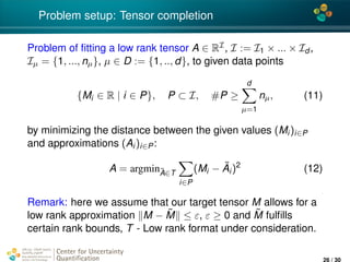
Example: updating of the solution u
0 0.5 1
-20
0
20
40
60
0 0.5 1
-20
0
20
40
60
0 0.5 1
-20
0
20
40
60
0 0.5 1
-20
0
20
40
60
0 0.5 1
-20
0
20
40
60
Figure: Original and updated solutions, mean value plus/minus 1,2,3
standard deviations. Number of available measurements {0, 1, 2, 3, 5}
[graphics are built in the stochastic Galerkin library sglib, written by E. Zander in TU Braunschweig]
Center for Uncertainty
Quantification
ation Logo Lock-up
29 / 30

32. 4*
Conclusion
Introduced low-rank tensor methods to solve elliptic PDEs
with uncertain coefficients,
Explained how to compute the maximum and the mean in
low-rank tensor format,
Derived Bayesian update surrogate ϕ (as a linear,
quadratic, cubic etc approximation), i.e. compute
conditional expectation of q, given measurement y.
Apply Tensor Completion method to sparse measurement
tensor in the likelihood.
Center for Uncertainty
Quantification
ation Logo Lock-up
30 / 30