Download as PDF, PPTX


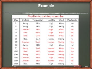
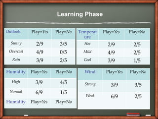
![Instance
Test Phase
Given a new instance,
x’=(Outlook=Sunny, Temperature=Cool, Humidity=High,
Wind=Strong)
P(Outlook=Sunny|Play=Yes) = 2/9
P(Outlook=Sunny|Play=No) = 3/5
P(Temperature=Cool|Play=Yes) = 3/9
P(Temperature=Cool|Play==No) = 1/5
P(Huminity=High|Play=Yes) = 3/9
P(Huminity=High|Play=No) = 4/5
P(Wind=Strong|Play=Yes) = 3/9
P(Wind=Strong|Play=No) = 3/5
P(Play=Yes) = 9/14
P(Play=No) = 5/14
P(Yes|x’): *P(Sunny|Yes)P(Cool|Yes)P(High|Yes)P(Strong|Yes)]P(Play=Yes) = 0.0053
P(No|x’): *P(Sunny|No) P(Cool|No)P(High|No)P(Strong|No)]P(Play=No) = 0.0206
Given the fact P(Yes|x’) < P(No|x’), we label x’ to be “No”.](https://image.slidesharecdn.com/dwdmnaivebayesankitgadgil027-121024125634-phpapp01/85/Dwdm-naive-bayes_ankit_gadgil_027-9-320.jpg)


This document discusses Naive Bayes classification. It begins by introducing classification and defining Naive Bayes as a simple probabilistic classifier based on applying Bayes' theorem with strong independent assumptions. It then provides an example of using Naive Bayes for classification, showing the learning and testing phases. It concludes that Naive Bayes is an intuitive and fast classification method that is widely used, particularly in fields like natural language processing.