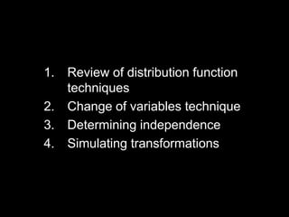
- The quiz will be handed out and start at 1pm, finishing at 1:10pm. - Though it is not for a grade, the instructor will collect the completed quizzes.

1. Quiz
• Pick up quiz and handout on your way in.
• Start at 1pm
• Finish at 1:10pm
• The quiz is not for a grade, but I will be
collecting it.

2. Stat 310
Bivariate Change of Variables
Garrett Grolemund

3. 1. Review of distribution function
techniques
2. Change of variables technique
3. Determining independence
4. Simulating transformations

4. Lakers' final scores

5. Laker's
Mean
87.2
Opponent's
Mean
81.2

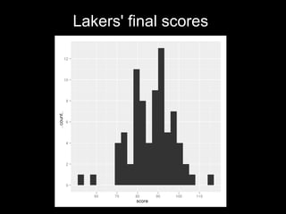
6. Let
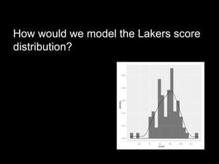
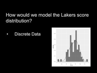
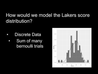
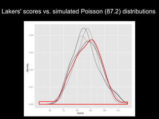
X = The Lakers' Score
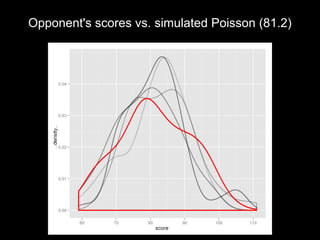
Y = The opponent's score
U = X -Y
Then the Lakers will win if U is positive,
and they will lose if U is negative.
How can we model U? (i.e, How can we
find the CDF and PDF of U?)

7. Recall from Tuesday
U = X - Y is a bivariate transformation
The Distribution function technique gives
us two ways to model X - Y:

8. 1. Begin with FX,Y(a):
Compute FU(a) in terms of FX,Y(a) by
equating probabilities

9. 1. Begin with FX,Y(a):
Compute FU(a) in terms of FX,Y(a) by
equating probabilities
FU(a) = P(U < a)
= P(X - Y < a)
= P(X < Y + a)
=?

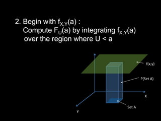
10. 2. Begin with fX,Y(a) :
Compute FU(a) by integrating fX,Y(a)
over the region where U < a
f(x,y)
P(Set A)
X
Set A
Y

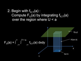
11. 2. Begin with fX,Y(a) :
Compute FU(a) by integrating fX,Y(a)
over the region where U < a
f(x,y)
∞ Y+a P(Set A)
FU(a) = ∫ ∫ fX,Y(a) dxdy
-∞ -∞
X
Set A
Y

12. Change of variables

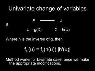
13. Univariate change of variables
X U
If
U = g(X) X = h(U)
Where h is the inverse of g, then
fU(u) = fx(h(u)) |h'(u)|
Method works for bivariate case, once we make
the appropriate modifications.

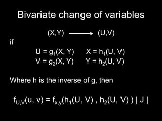
14. Bivariate change of variables
(X,Y) (U,V)
if
U = g1(X, Y) X = h1(U, V)
V = g2(X, Y) Y = h2(U, V)
Where h is the inverse of g, then
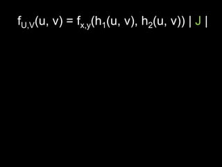
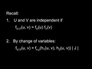
fU,V(u, v) = fx,y(h1(U, V) , h2(U, V) ) | J |

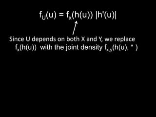
15. fU(u) = fx(h(u)) |h'(u)|
Since U depends on both X and Y, we replace
fx(h(u)) with the joint density fx,y(h(u), * )

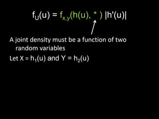
16. fU(u) = fx,y(h(u), * ) |h'(u)|
A joint density must be a function of two
random variables
Let X = h1(u) and Y = h2(u)

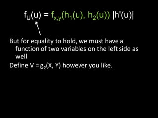
17. fU(u) = fx,y(h1(u), h2(u)) |h'(u)|
But for equality to hold, we must have a
function of two variables on the left side as
well
Define V = g2(X, Y) however you like.

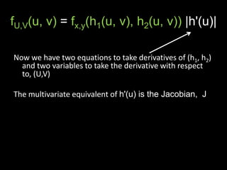
18. fU,V(u, v) = fx,y(h1(u, v), h2(u, v)) |h'(u)|
Now we have two equations to take derivatives of (h1, h2)
and two variables to take the derivative with respect
to, (U,V)
The multivariate equivalent of h'(u) is the Jacobian, J

19. fU,V(u, v) = fx,y(h1(u, v), h2(u, v)) | J |
And we're finished

20. Jacobian
δx δx
δu δv
J=
δy δy
δu δv

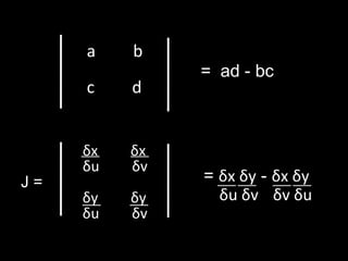
21. a b
= ad - bc
c d
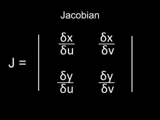
δx δx
δu δv
J= = δx δy - δx δy
δy δy δu δv δv δu
δu δv

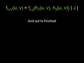
22. fU,V(u, v) = fx,y(h1(u, v), h2(u, v)) | J |
U=X-Y
What should V be?

23. fU,V(u, v) = fx,y(h1(u, v), h2(u, v)) | J |
U=X-Y
What should V be?
• Sometimes we want V to be something specific
• Otherwise keep V simple or helpful
e.g., V = Y

24. fU,V(u, v) = fx,y(h1(u, v), h2(u, v)) | J |
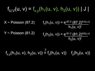
What should fx,y(*, *) be?

25. fU,V(u, v) = fx,y(h1(u, v), h2(u, v)) | J |
What should fx,y(*, *) be?
First consider: what should fx(*) and fy(*) be?

26. How would we model the Lakers score
distribution?

27. How would we model the Lakers score
distribution?
• Discrete Data

28. How would we model the Lakers score
distribution?
• Discrete Data
• Sum of many
bernoulli trials

29. How would we model the Lakers score
distribution?
• Discrete Data
• Sum of many
bernoulli trials
Poisson?

30. Lakers' scores vs. simulated Poisson (87.2) distributions

31. Opponent's scores vs. simulated Poisson (81.2)

32. fU,V(u, v) = fx,y(h1(u, v), h2(u, v)) | J |
X ~ Poisson (87.2) fx(h1(u, v)) = e-87.2 (87.2)h1(u,v)
h1(u, v)!
Y ~ Poisson (81.2) fy(h2(u, v)) = e-81.2 (81.2)h2(u,v)
h2(u, v)!
?
fx,y(h1(u, v), h2(u, v)) = fx(h1(u, v)) fy(h2(u, v))

33. ρ = 0.412

34. fU,V(u, v) = fx,y(h1(u, v), h2(u, v)) | J |

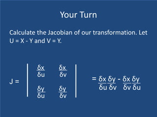
35. Your Turn
Calculate the Jacobian of our transformation. Let
U = X - Y and V = Y.
δx δx
δu δv
J= = δx δy - δx δy
δy δy δu δv δv δu
δu δv

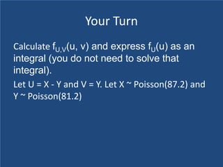
36. Your Turn
Calculate fU,V(u, v) and express fU(u) as an
integral (you do not need to solve that
integral).
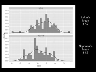
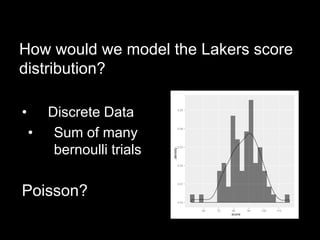
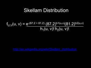
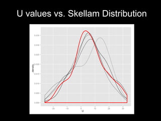
Let U = X - Y and V = Y. Let X ~ Poisson(87.2) and
Y ~ Poisson(81.2)

37. Skellam Distribution
fU,V(u, v) = e-(87.2 + 81.2) (87.2)h1(u,v)(81.2)h2(u,v)
h1(u, v)! h2(u, v)!
http://en.wikipedia.org/wiki/Skellam_distribution

38. U values

39. U values vs. Skellam Distribution

40. Testing Independence

41. Recall:
1. U and V are independent if
fU,V(u, v) = fU(u) fV(v)
2. By change of variables:
fU,V(u, v) = fx,y(h1(u, v), h2(u, v)) | J |

42. Complete the proof
Complete the handout to show that U = X + Y and
V = X - Y are independent when X, Y ~ N(0, 1).

43. Simulation

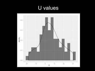
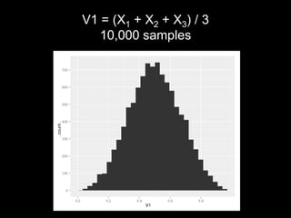
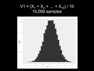
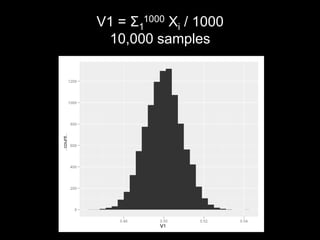
44. We can also learn a lot about the distribution of
a random variable by simulating it.
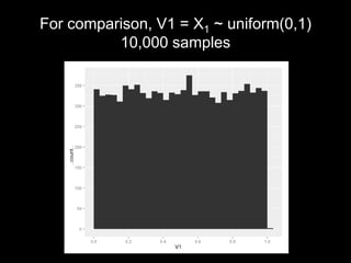
Let Xi ~ Uniform (0,1)
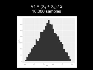
Let U = (X1 + X2 ) / 2
If we generate a 100 pairs of X1 and X2 and plot
(X1 + X2 ) / 2 for each pair, we will have a
simulation of the distribution of U

45. For comparison, V1 = X1 ~ uniform(0,1)
10,000 samples

46. V1 = (X1 + X2) / 2
10,000 samples

47. V1 = (X1 + X2 + X3) / 3
10,000 samples

48. V1 = (X1 + X2 + … + X10) / 10
10,000 samples

49. V1 = Σ11000 Xi / 1000
10,000 samples