
Downloaded 873 times

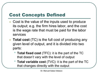
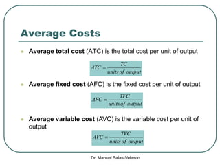
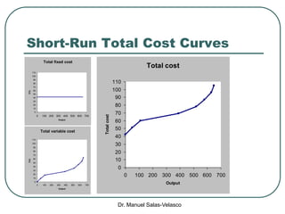
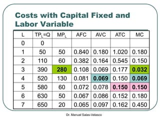
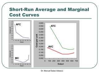
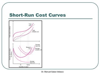
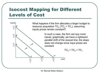
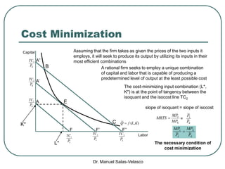
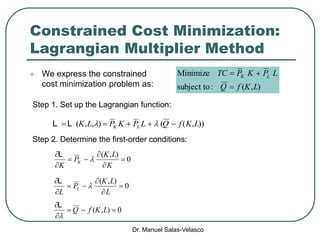
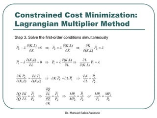
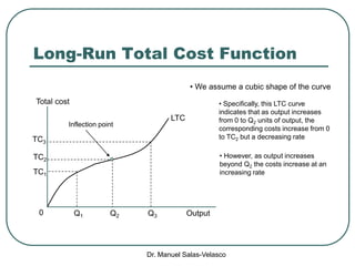
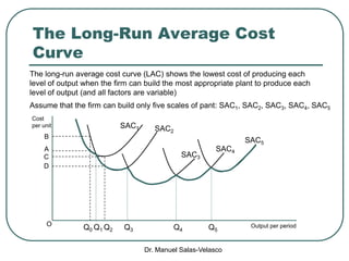
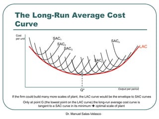
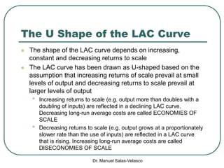
The document discusses cost functions, distinguishing between total, fixed, and variable costs, along with average costs, marginal costs, and short-run and long-run cost variations. It details how input prices influence production functions, the cost-minimization process using the Lagrangian multiplier method, and the formation of cost curves in both short and long runs. Finally, it explains the concept of the long-run average cost curve and its U-shape, highlighting the relationship with returns to scale.


