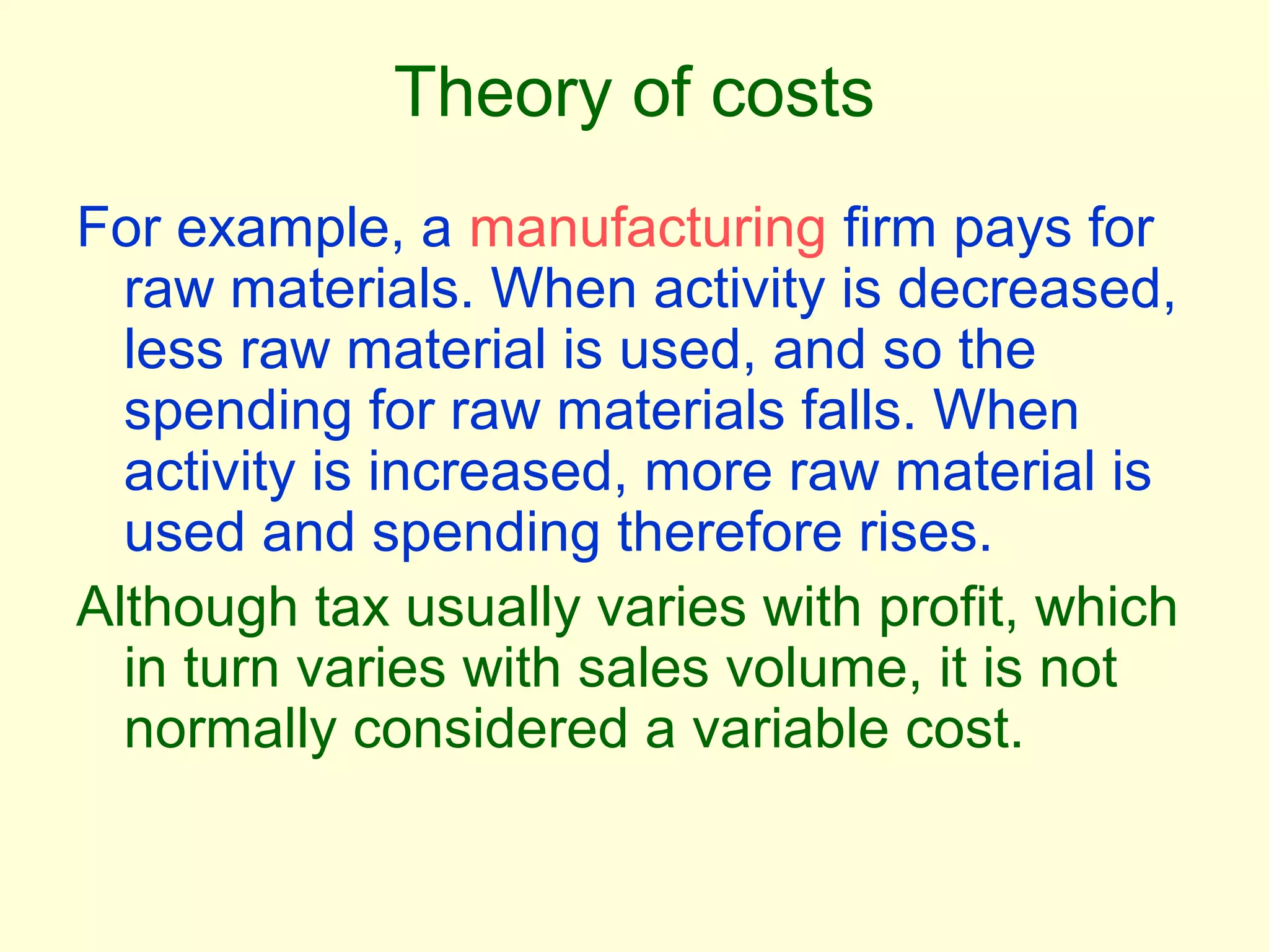
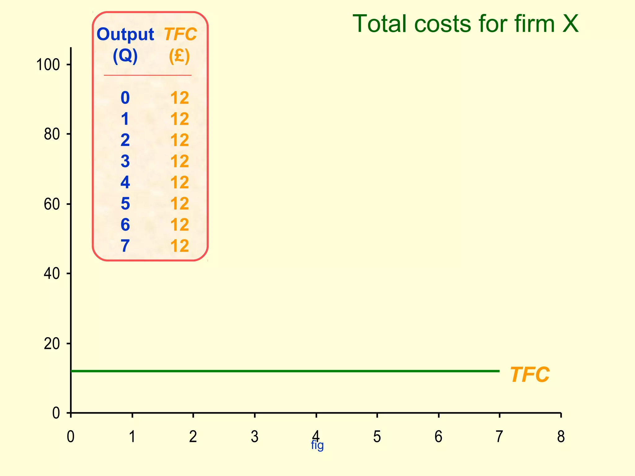
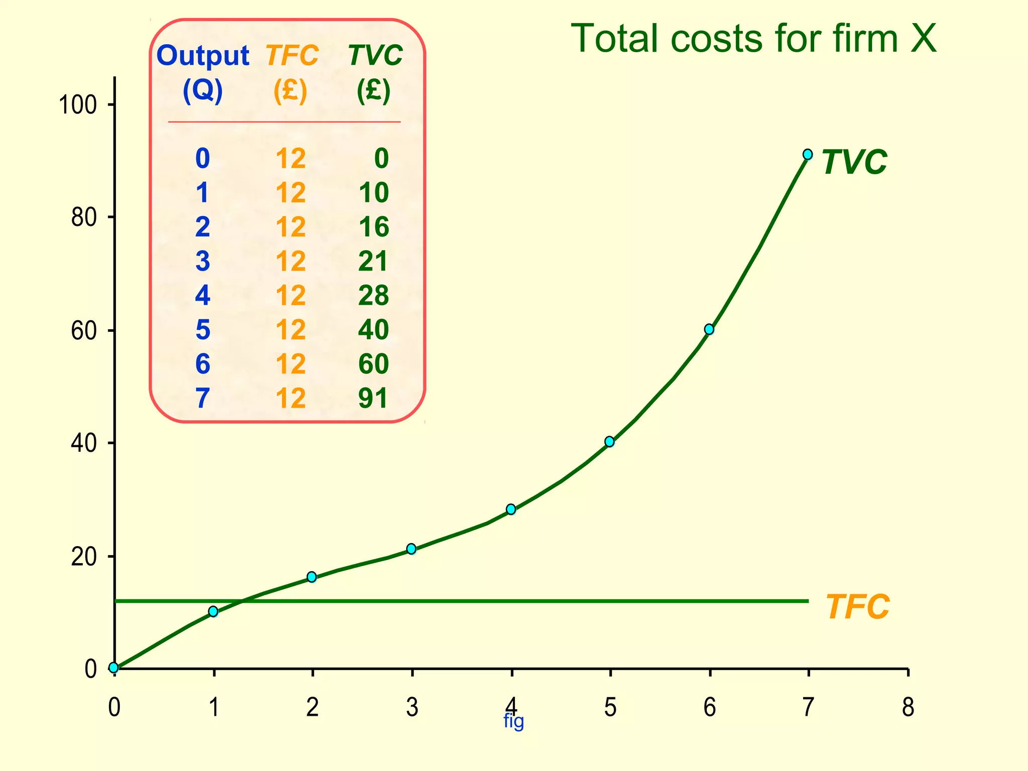
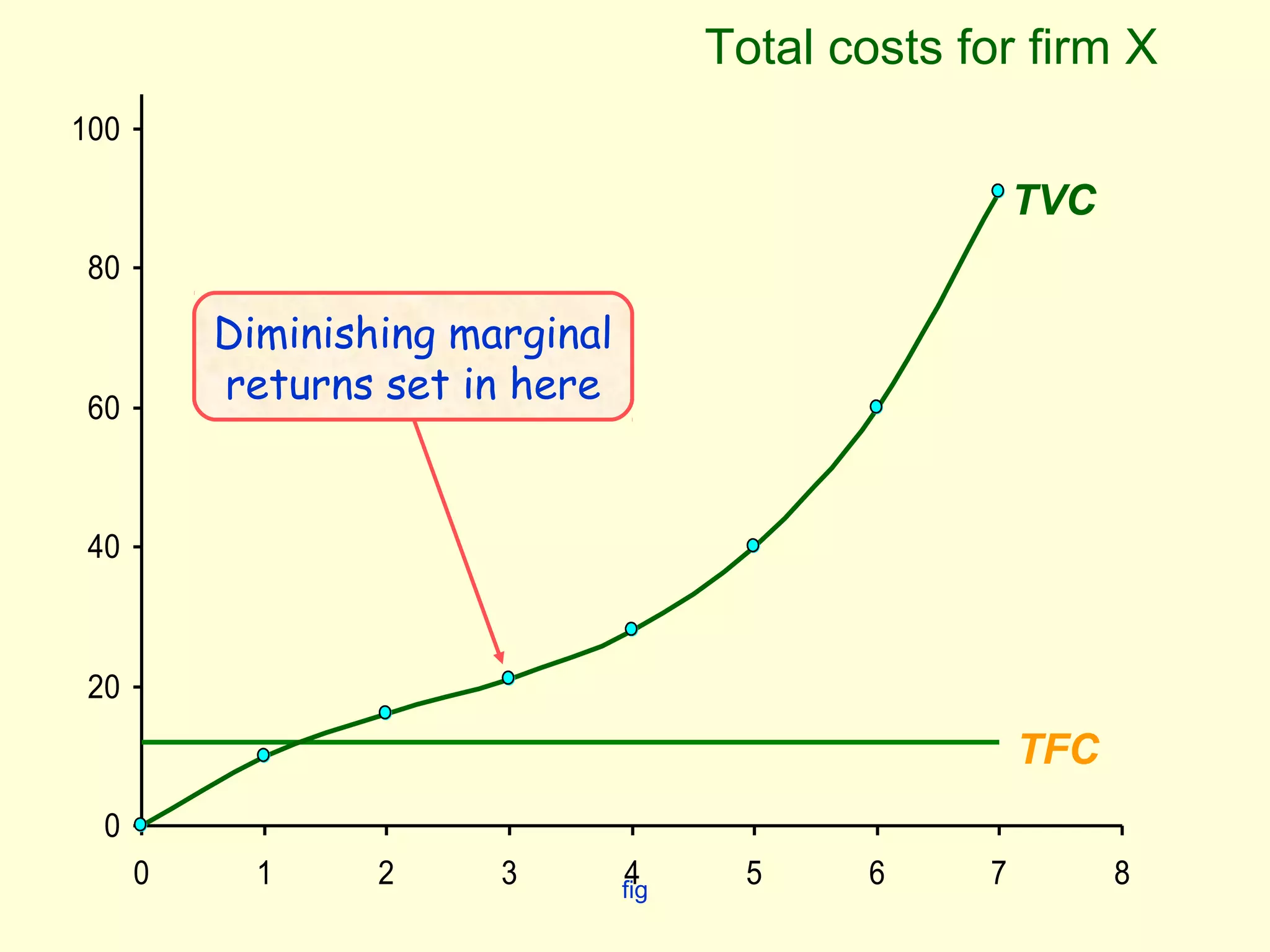
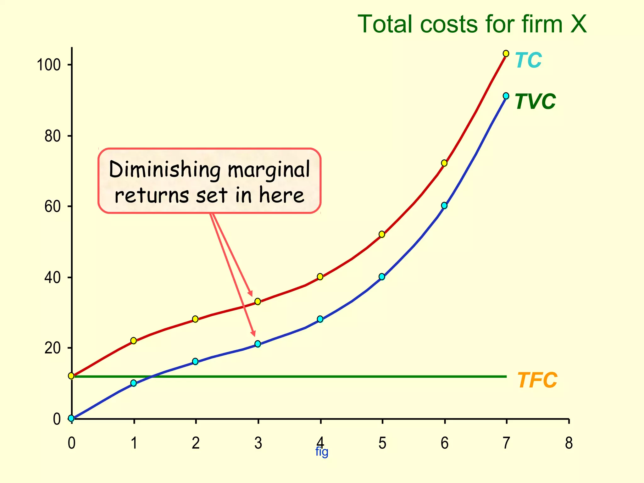
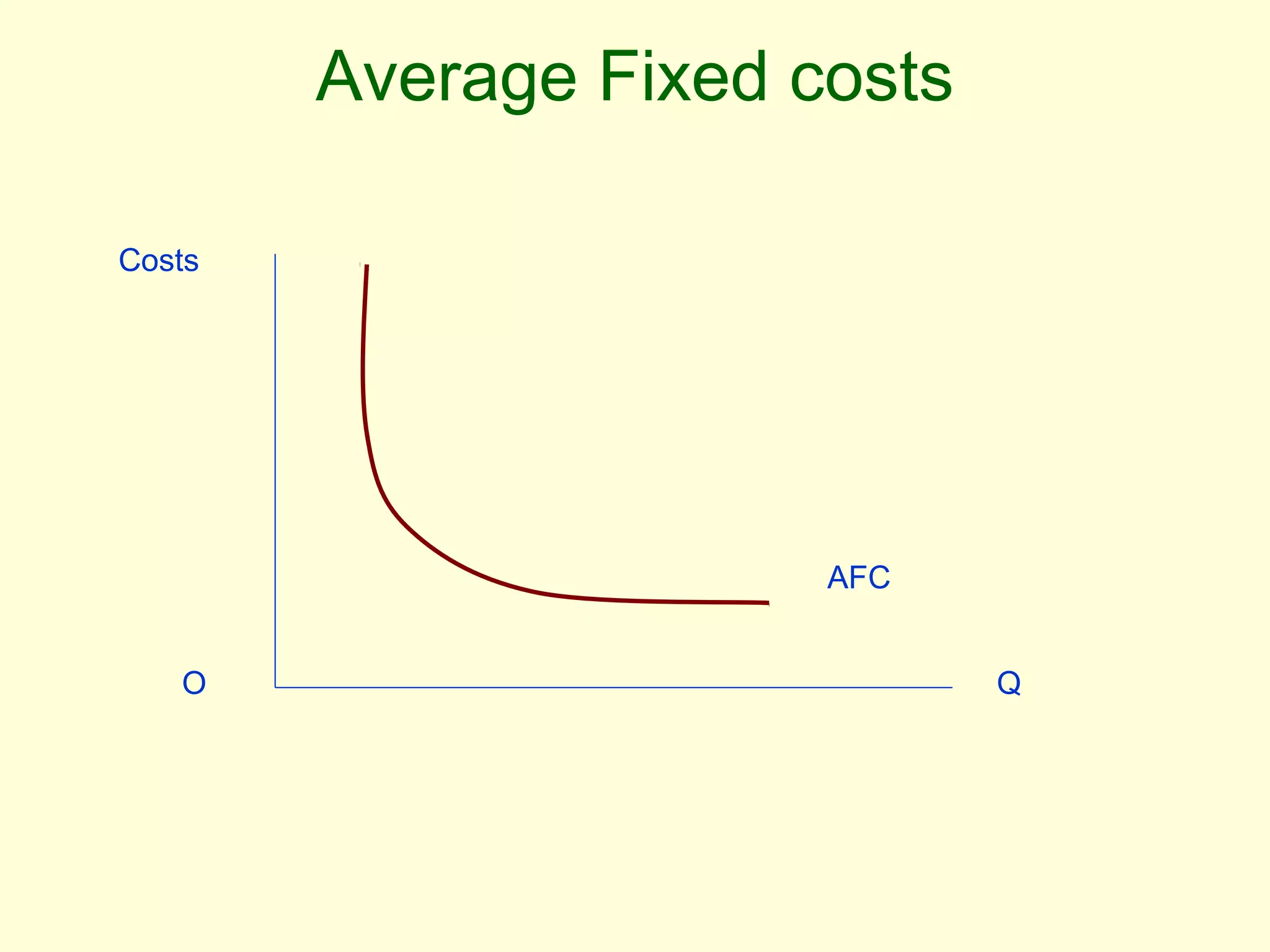
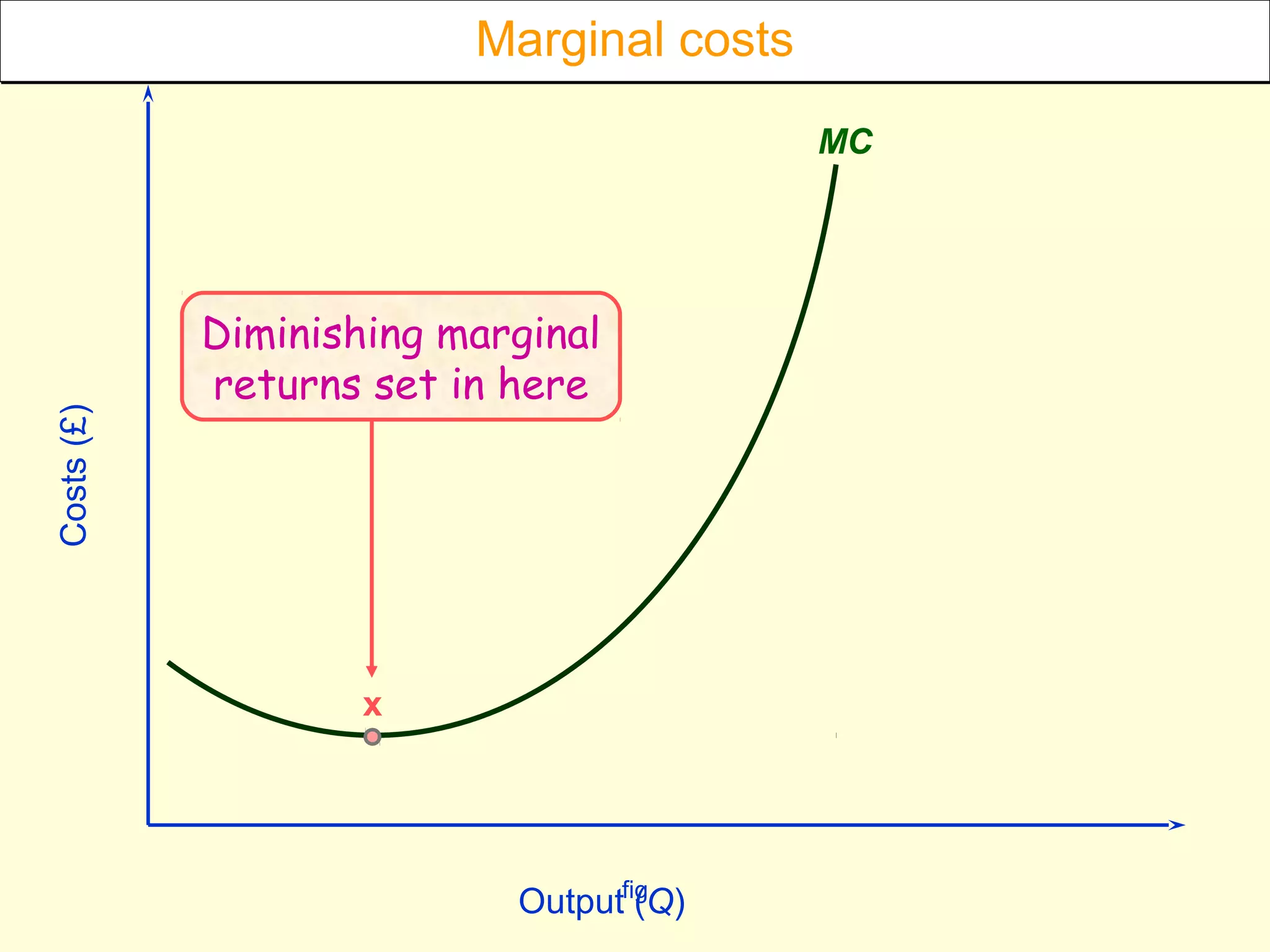
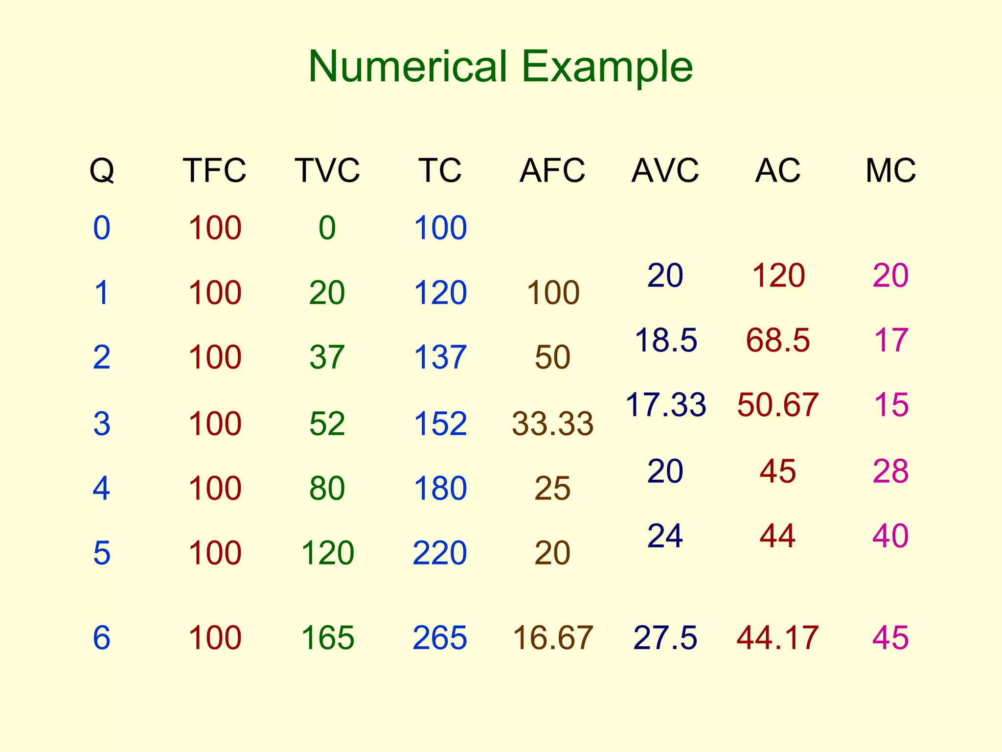
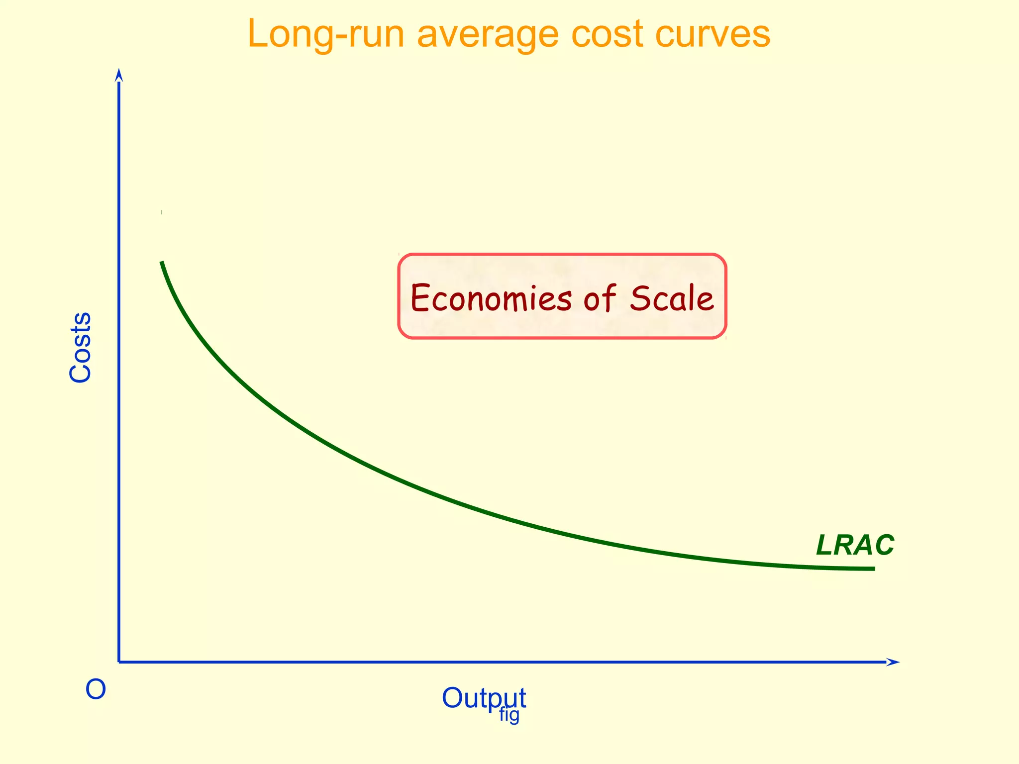
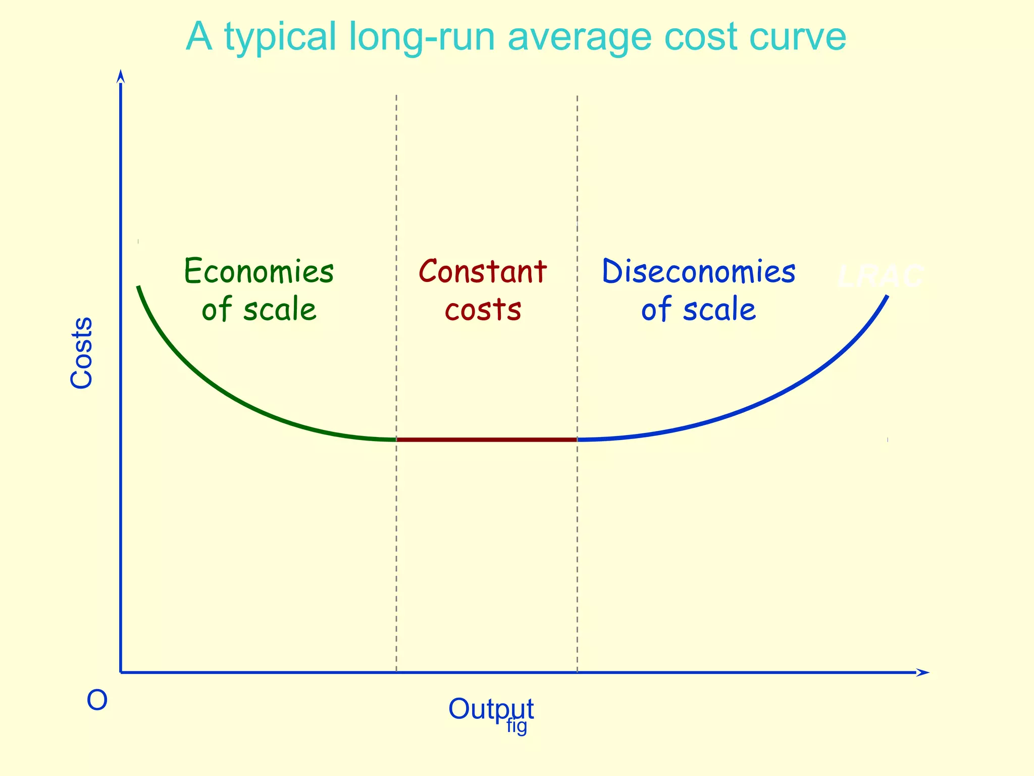
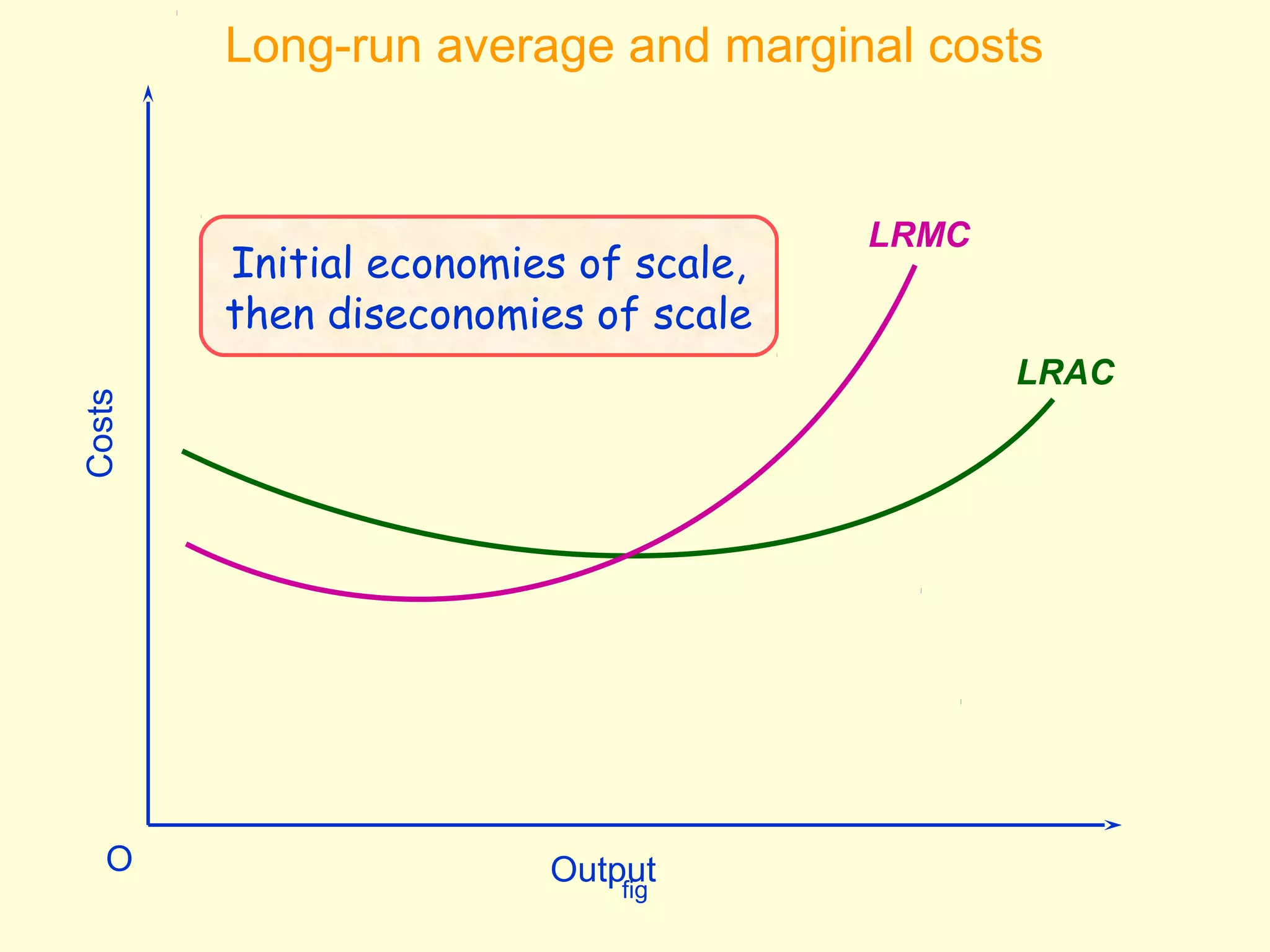
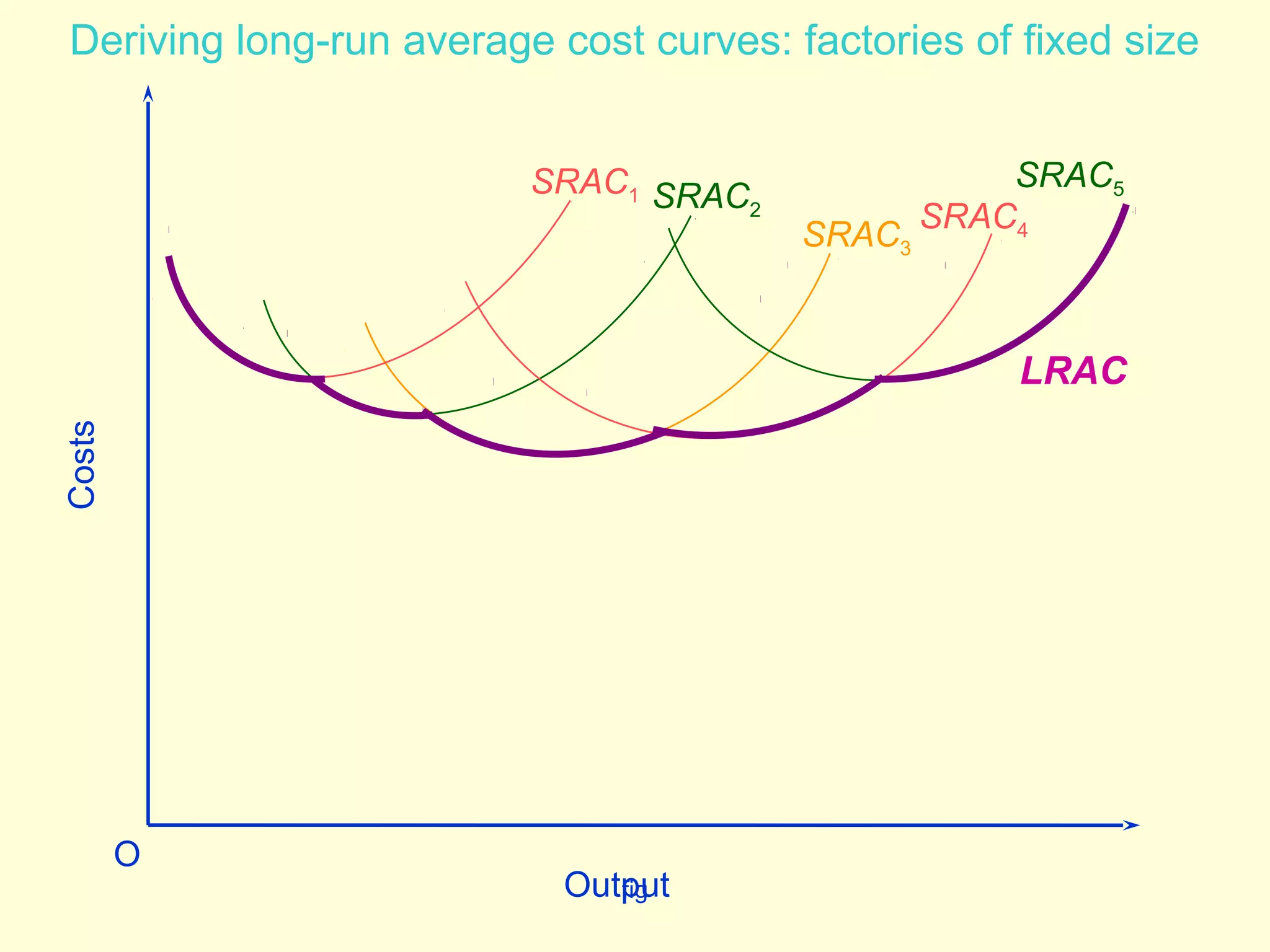
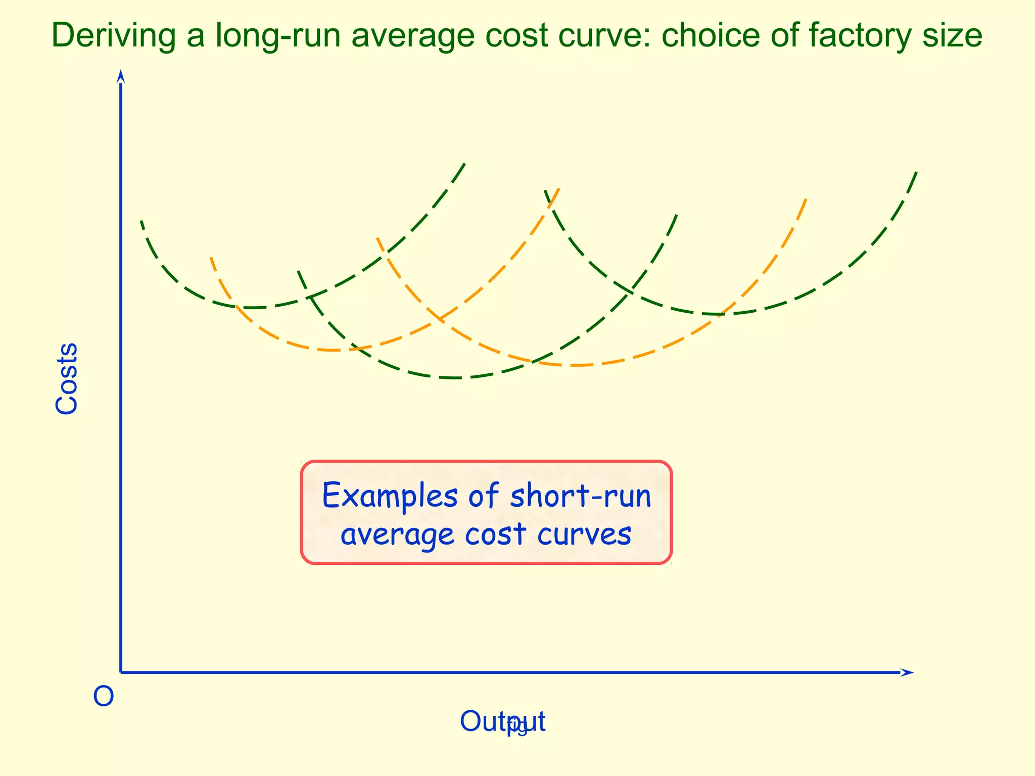
THEORY OF COSTS 
Short Run
Decision making in different time 
periods 
 Short run for the firms and very short run for 
the industry. 
 Long run for the firms and short run for the 
industry. 
 Very long run for the firms and long run for the 
industry.
Theory of costs 
• Costs of a firm is incurred to establish the 
production unit and to purchase different 
factors of production. 
• Cost of a firm (TC) is classified into two 
broad categories - Fixed cost (TFC) and 
Variable cost (TVC). 
i.e. TC = TFC + TVC 
• However, nothing is fixed in the long run.
Theory of costs 
Fixed costs 
Fixed costs are expenses that does not 
change in proportion to the activity of a 
business. 
Fixed costs include overheads (rent, 
insurance-premium, interests), and also 
direct costs such as payroll (particularly 
salaries).
Theory of costs 
Fixed cost does not change with the 
volume of production. 
TFC 
Q 
costs 
100 
O
Theory of costs 
Variable costs 
Variable costs change in direct 
proportion to the activity of a business 
such as sales or production volume. In 
retail, the cost of goods is almost entirely 
variable. In manufacturing, direct material 
costs, wages, fuel costs are examples of 
variable costs.
Theory of costs 
For example, a manufacturing firm pays for 
raw materials. When activity is decreased, 
less raw material is used, and so the 
spending for raw materials falls. When 
activity is increased, more raw material is 
used and spending therefore rises. 
Although tax usually varies with profit, which 
in turn varies with sales volume, it is not 
normally considered a variable cost.
fig 
100 
80 
60 
40 
20 
0 
Total costs for firm X 
TFC 
Output 
(Q) 
01234567 
TFC 
(£) 
12 
12 
12 
12 
12 
12 
12 
12 
0 1 2 3 4 5 6 7 8
fig 
100 
80 
60 
40 
20 
0 
Total costs for firm X 
TFC 
Output 
(Q) 
01234567 
TFC 
(£) 
12 
12 
12 
12 
12 
12 
12 
12 
TVC 
(£) 
0 
10 
16 
21 
28 
40 
60 
91 
0 1 2 3 4 5 6 7 8
fig 
100 
80 
60 
40 
20 
0 
Total costs for firm X 
TVC 
Output 
(Q) 
01234567 
TFC 
(£) 
12 
12 
12 
12 
12 
12 
12 
12 
TVC 
(£) 
0 
10 
16 
21 
28 
40 
60 
91 
TFC 
0 1 2 3 4 5 6 7 8
fig 
100 
80 
60 
40 
20 
0 
Total costs for firm X 
TVC 
TFC 
Diminishing marginal 
returns set in here 
0 1 2 3 4 5 6 7 8
fig 
100 
80 
60 
40 
20 
0 
Total costs for firm X 
TVC 
Output 
(Q) 
01234567 
TFC 
(£) 
12 
12 
12 
12 
12 
12 
12 
12 
TVC 
(£) 
0 
10 
16 
21 
28 
40 
60 
91 
TFC 
0 1 2 3 4 5 6 7 8
fig 
100 
80 
60 
40 
20 
0 
Total costs for firm X 
TVC 
TFC 
Output 
(Q) 
01234567 
TFC 
(£) 
12 
12 
12 
12 
12 
12 
12 
12 
TVC 
(£) 
0 
10 
16 
21 
28 
40 
60 
91 
TC 
(£) 
12 
22 
28 
33 
40 
52 
72 
103 
0 1 2 3 4 5 6 7 8
fig 
100 
80 
60 
40 
20 
0 
Total costs for firm X 
TC 
Output 
(Q) 
01234567 
TFC 
(£) 
12 
12 
12 
12 
12 
12 
12 
12 
TVC 
(£) 
0 
10 
16 
21 
28 
40 
60 
91 
TC 
(£) 
12 
22 
28 
33 
40 
52 
72 
103 
TVC 
TFC 
0 1 2 3 4 5 6 7 8
fig 
100 
80 
60 
40 
20 
0 
Total costs for firm X 
TC 
TVC 
TFC 
Diminishing marginal 
returns set in here 
0 1 2 3 4 5 6 7 8
Average fixed cost 
Average fixed cost (AFC) = TFC/Q 
where TFC = fixed cost, Q = total number of 
units produced. 
Unit fixed costs decline along with volume, 
following a rectangular hyperbola. As a 
result, the total unit cost of a product will 
decline as volume increases.
Average Fixed costs 
Q 
Costs 
AFC 
O
Average variable cost 
Average variable cost (AVC) is the TVC of a firm 
divided by the total units of output (Q). 
AVC = TVC/Q 
Q 
costs 
Y 
AVC 
O
Average cost 
Average cost (AC) is the TC of a firm divided by 
the total units of output (Q). 
AC = TC/Q = AFC + AVC 
Q 
costs 
Z 
AC 
O
Marginal Cost 
The additional cost incurred to produce one 
additional unit of output is called the 
Marginal Cost (MC). 
MC = dC/dQ
MC 
The marginal cost curve is U-shaped. 
Marginal cost is relatively high at small 
quantities of output - then as production 
increases, it declines - then reaches a 
minimum value - then rises. 
This shape of the marginal cost curve is 
directly attributable to increasing, then 
decreasing marginal returns (the law of 
diminishing marginal returns).
Diminishing marginal 
returns set in here 
fig Output (Q) Costs (£) 
MC 
x 
MMaarrggiinnaall ccoossttss
Numerical Example 
Q TFC TVC TC AFC AVC AC MC 
0 100 0 100 
1 100 20 120 100 20 120 20 
2 100 37 137 50 18.5 68.5 17 
3 100 52 152 33.33 17.33 50.67 15 
4 100 80 180 25 20 45 28 
5 100 120 220 20 24 44 40 
6 100 165 265 16.67 27.5 44.17 45
Average and marginal costs 
fig Output (Q) Costs (£) 
AVC 
AFC 
MC 
x 
AC 
z 
y
LONG RUN
Long run cost curves 
The Long run average cost (LRAC or LAC) 
curve illustrates - for a given quantity of 
production - the average cost per unit 
which a firm faces in the long run (i.e. 
when no factors of production is fixed).
LRAC 
LRAC curve is derived from a series of short 
run average cost curves. 
It is also called the ‘Envelope curve' since it 
envelops all the short run average cost 
curve. 
The curve is created as an envelope of an 
infinite number of short-run average total 
cost curves.
LAC 
The LRAC curve is U-shaped, reflecting 
economies of scale when it is negatively-sloped 
and diseconomies of scale when it 
is positively sloped. 
In perfect competition, the LRAC curve is 
flat at the point of equilibrium – in this 
stage the firm is enjoying constant returns 
to scale.
LAC 
In some industries, the LRAC is L-shaped, 
and economies of scale increase 
indefinitely. This means that the largest 
firm tends to have a cost advantage, and 
the industry tends naturally to become a 
monopoly, and hence is called a natural 
monopoly. Natural monopolies tend to 
exist in industries with high capital costs in 
relation to variable costs, such as water 
supply and electricity supply.
Long-run average cost curves 
Output OCosts 
fig 
LRAC 
Economies of Scale
long-run average cost curves 
fig Output OCosts 
LRAC 
Diseconomies of Scale
long-run average cost curves 
fig Output OCosts 
LRAC 
Constant costs
Long-run Costs 
• Long-run average costs 
– assumptions behind the curve 
• factor prices are give 
• state of technology and factor quality are given 
• firms choose least-cost combination of factors
A typical long-run average cost curve 
Output OCosts 
fig 
LRAC
A typical long-run average cost curve 
Economies Constant 
LRAC 
of scale 
costs 
fig Output OCosts 
Diseconomies 
of scale
Long-run Costs 
• Long-run average costs 
– assumptions behind the curve 
• factor prices are give 
• state of technology and factor quality are given 
• firms choose least-cost combination of factors 
– shape of the LRAC curve 
– a typical LRAC curve 
– long-run average and marginal cost curves
Long-run average and marginal costs 
Output OCosts 
fig 
LRAC 
LRMC 
Economies of Scale
Long-run average and marginal costs 
fig Output OCosts 
LRMC 
LRAC 
Diseconomies of Scale
Long-run average and marginal costs 
fig Output OCosts 
LRAC = LRMC 
Constant costs
Long-run average and marginal costs 
fig Output OCosts 
LRMC 
LRAC 
Initial economies of scale, 
then diseconomies of scale
Long-run Costs 
• Long-run average costs 
– assumptions behind the curve 
• factor prices are given. 
• state of technology and factor quality are 
given. 
• firms choose least-cost combination of 
factors.
Envelope Curve 
The envelope curve is based on the point of 
each short-run ATC curve that provides 
the lowest possible average cost for each 
quantity of output.
Deriving long-run average cost curves: plants of fixed size 
fig 
SRAC3 
1 factory 
Costs Output 
O 
SRAC5 
SRAC4 
5 factories 
4 factories 
3 factories 
2 factories 
SRAC1 SRAC2
Deriving long-run average cost curves: factories of fixed size 
SRAC1 
fig 
SRAC2 SRAC4 
SRAC3 
SRAC5 
LRAC 
Costs Output 
O
Deriving a long-run average cost curve: choice of factory size 
Costs Output 
fig 
O 
Examples of short-run 
average cost curves
Deriving a long-run average cost curve: choice of factory size 
fig 
LRAC 
Costs Output 
O

Cost 3

  • 1.
    THEORY OF COSTS Short Run
  • 2.
    Decision making indifferent time periods  Short run for the firms and very short run for the industry.  Long run for the firms and short run for the industry.  Very long run for the firms and long run for the industry.
  • 3.
    Theory of costs • Costs of a firm is incurred to establish the production unit and to purchase different factors of production. • Cost of a firm (TC) is classified into two broad categories - Fixed cost (TFC) and Variable cost (TVC). i.e. TC = TFC + TVC • However, nothing is fixed in the long run.
  • 4.
    Theory of costs Fixed costs Fixed costs are expenses that does not change in proportion to the activity of a business. Fixed costs include overheads (rent, insurance-premium, interests), and also direct costs such as payroll (particularly salaries).
  • 5.
    Theory of costs Fixed cost does not change with the volume of production. TFC Q costs 100 O
  • 6.
    Theory of costs Variable costs Variable costs change in direct proportion to the activity of a business such as sales or production volume. In retail, the cost of goods is almost entirely variable. In manufacturing, direct material costs, wages, fuel costs are examples of variable costs.
  • 7.
    Theory of costs For example, a manufacturing firm pays for raw materials. When activity is decreased, less raw material is used, and so the spending for raw materials falls. When activity is increased, more raw material is used and spending therefore rises. Although tax usually varies with profit, which in turn varies with sales volume, it is not normally considered a variable cost.
  • 8.
    fig 100 80 60 40 20 0 Total costs for firm X TFC Output (Q) 01234567 TFC (£) 12 12 12 12 12 12 12 12 0 1 2 3 4 5 6 7 8
  • 9.
    fig 100 80 60 40 20 0 Total costs for firm X TFC Output (Q) 01234567 TFC (£) 12 12 12 12 12 12 12 12 TVC (£) 0 10 16 21 28 40 60 91 0 1 2 3 4 5 6 7 8
  • 10.
    fig 100 80 60 40 20 0 Total costs for firm X TVC Output (Q) 01234567 TFC (£) 12 12 12 12 12 12 12 12 TVC (£) 0 10 16 21 28 40 60 91 TFC 0 1 2 3 4 5 6 7 8
  • 11.
    fig 100 80 60 40 20 0 Total costs for firm X TVC TFC Diminishing marginal returns set in here 0 1 2 3 4 5 6 7 8
  • 12.
    fig 100 80 60 40 20 0 Total costs for firm X TVC Output (Q) 01234567 TFC (£) 12 12 12 12 12 12 12 12 TVC (£) 0 10 16 21 28 40 60 91 TFC 0 1 2 3 4 5 6 7 8
  • 13.
    fig 100 80 60 40 20 0 Total costs for firm X TVC TFC Output (Q) 01234567 TFC (£) 12 12 12 12 12 12 12 12 TVC (£) 0 10 16 21 28 40 60 91 TC (£) 12 22 28 33 40 52 72 103 0 1 2 3 4 5 6 7 8
  • 14.
    fig 100 80 60 40 20 0 Total costs for firm X TC Output (Q) 01234567 TFC (£) 12 12 12 12 12 12 12 12 TVC (£) 0 10 16 21 28 40 60 91 TC (£) 12 22 28 33 40 52 72 103 TVC TFC 0 1 2 3 4 5 6 7 8
  • 15.
    fig 100 80 60 40 20 0 Total costs for firm X TC TVC TFC Diminishing marginal returns set in here 0 1 2 3 4 5 6 7 8
  • 16.
    Average fixed cost Average fixed cost (AFC) = TFC/Q where TFC = fixed cost, Q = total number of units produced. Unit fixed costs decline along with volume, following a rectangular hyperbola. As a result, the total unit cost of a product will decline as volume increases.
  • 17.
    Average Fixed costs Q Costs AFC O
  • 18.
    Average variable cost Average variable cost (AVC) is the TVC of a firm divided by the total units of output (Q). AVC = TVC/Q Q costs Y AVC O
  • 19.
    Average cost Averagecost (AC) is the TC of a firm divided by the total units of output (Q). AC = TC/Q = AFC + AVC Q costs Z AC O
  • 20.
    Marginal Cost Theadditional cost incurred to produce one additional unit of output is called the Marginal Cost (MC). MC = dC/dQ
  • 21.
    MC The marginalcost curve is U-shaped. Marginal cost is relatively high at small quantities of output - then as production increases, it declines - then reaches a minimum value - then rises. This shape of the marginal cost curve is directly attributable to increasing, then decreasing marginal returns (the law of diminishing marginal returns).
  • 22.
    Diminishing marginal returnsset in here fig Output (Q) Costs (£) MC x MMaarrggiinnaall ccoossttss
  • 23.
    Numerical Example QTFC TVC TC AFC AVC AC MC 0 100 0 100 1 100 20 120 100 20 120 20 2 100 37 137 50 18.5 68.5 17 3 100 52 152 33.33 17.33 50.67 15 4 100 80 180 25 20 45 28 5 100 120 220 20 24 44 40 6 100 165 265 16.67 27.5 44.17 45
  • 24.
    Average and marginalcosts fig Output (Q) Costs (£) AVC AFC MC x AC z y
  • 25.
  • 26.
    Long run costcurves The Long run average cost (LRAC or LAC) curve illustrates - for a given quantity of production - the average cost per unit which a firm faces in the long run (i.e. when no factors of production is fixed).
  • 27.
    LRAC LRAC curveis derived from a series of short run average cost curves. It is also called the ‘Envelope curve' since it envelops all the short run average cost curve. The curve is created as an envelope of an infinite number of short-run average total cost curves.
  • 28.
    LAC The LRACcurve is U-shaped, reflecting economies of scale when it is negatively-sloped and diseconomies of scale when it is positively sloped. In perfect competition, the LRAC curve is flat at the point of equilibrium – in this stage the firm is enjoying constant returns to scale.
  • 29.
    LAC In someindustries, the LRAC is L-shaped, and economies of scale increase indefinitely. This means that the largest firm tends to have a cost advantage, and the industry tends naturally to become a monopoly, and hence is called a natural monopoly. Natural monopolies tend to exist in industries with high capital costs in relation to variable costs, such as water supply and electricity supply.
  • 30.
    Long-run average costcurves Output OCosts fig LRAC Economies of Scale
  • 31.
    long-run average costcurves fig Output OCosts LRAC Diseconomies of Scale
  • 32.
    long-run average costcurves fig Output OCosts LRAC Constant costs
  • 33.
    Long-run Costs •Long-run average costs – assumptions behind the curve • factor prices are give • state of technology and factor quality are given • firms choose least-cost combination of factors
  • 34.
    A typical long-runaverage cost curve Output OCosts fig LRAC
  • 35.
    A typical long-runaverage cost curve Economies Constant LRAC of scale costs fig Output OCosts Diseconomies of scale
  • 36.
    Long-run Costs •Long-run average costs – assumptions behind the curve • factor prices are give • state of technology and factor quality are given • firms choose least-cost combination of factors – shape of the LRAC curve – a typical LRAC curve – long-run average and marginal cost curves
  • 37.
    Long-run average andmarginal costs Output OCosts fig LRAC LRMC Economies of Scale
  • 38.
    Long-run average andmarginal costs fig Output OCosts LRMC LRAC Diseconomies of Scale
  • 39.
    Long-run average andmarginal costs fig Output OCosts LRAC = LRMC Constant costs
  • 40.
    Long-run average andmarginal costs fig Output OCosts LRMC LRAC Initial economies of scale, then diseconomies of scale
  • 41.
    Long-run Costs •Long-run average costs – assumptions behind the curve • factor prices are given. • state of technology and factor quality are given. • firms choose least-cost combination of factors.
  • 42.
    Envelope Curve Theenvelope curve is based on the point of each short-run ATC curve that provides the lowest possible average cost for each quantity of output.
  • 43.
    Deriving long-run averagecost curves: plants of fixed size fig SRAC3 1 factory Costs Output O SRAC5 SRAC4 5 factories 4 factories 3 factories 2 factories SRAC1 SRAC2
  • 44.
    Deriving long-run averagecost curves: factories of fixed size SRAC1 fig SRAC2 SRAC4 SRAC3 SRAC5 LRAC Costs Output O
  • 45.
    Deriving a long-runaverage cost curve: choice of factory size Costs Output fig O Examples of short-run average cost curves
  • 46.
    Deriving a long-runaverage cost curve: choice of factory size fig LRAC Costs Output O