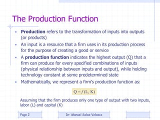
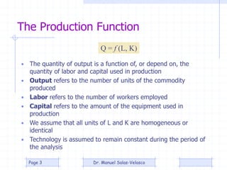
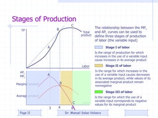
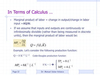
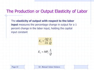
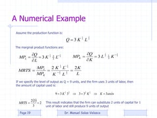
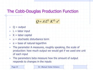
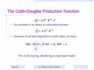
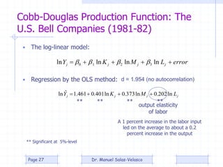
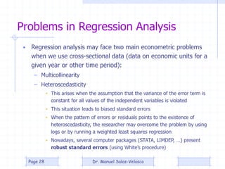
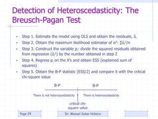
The document provides an overview of production theory, focusing on the production function which describes the relationship between inputs (labor and capital) and output. It discusses concepts like the short-run and long-run production, the law of diminishing returns, and the Cobb-Douglas production function, detailing how different variables affect production and efficiency. Additionally, it covers the econometric analysis of production functions, including the regression analysis challenges and methods to identify heteroscedasticity.

1. Production Theory
Dr. Manuel Salas-Velasco
University of Granada, Spain
Dr. Manuel Salas-VelascoPage 1

2. The Production Function
• Production refers to the transformation of inputs into outputs
(or products)
• An input is a resource that a firm uses in its production process
for the purpose of creating a good or service
• A production function indicates the highest output (Q) that a
firm can produce for every specified combinations of inputs
(physical relationship between inputs and output), while holding
technology constant at some predetermined state
• Mathematically, we represent a firm’s production function as:
Q = f (L, K)
Assuming that the firm produces only one type of output with two inputs,
labor (L) and capital (K)
Dr. Manuel Salas-VelascoPage 2

3. The Production Function
• The quantity of output is a function of, or depend on, the
quantity of labor and capital used in production
• Output refers to the number of units of the commodity
produced
• Labor refers to the number of workers employed
• Capital refers to the amount of the equipment used in
production
• We assume that all units of L and K are homogeneous or
identical
• Technology is assumed to remain constant during the period of
the analysis
Q = f (L, K)
Dr. Manuel Salas-VelascoPage 3

4. Production Theory
The Production Function in the
Short Run
Dr. Manuel Salas-VelascoPage 4

5. The Short Run
• The short run is a time period in which the quantity
of some inputs, called fixed factors, cannot be
increased. So, it does not correspond to a specific
number of months or years
• A fixed factor is usually an element of capital (such
as plant and equipment). Therefore, in our
production function capital is taken to be the fixed
factor and labor the variable one
),( KLfQ 
Dr. Manuel Salas-VelascoPage 5

6. Total, Average and Marginal Products
• Total product (TP) is the total amount that is
produced during a given period of time
• Total product will change as more or less of the
variable factor is used in conjunction with the given
amount of the fixed factor
• Average product (AP) is the total product divided by
the number of units of the variable factor used to
produce it
• Marginal product (MP) is the change in total product
resulting from the use of one additional unit of the
variable factor
Dr. Manuel Salas-VelascoPage 6

7. Output with Fixed Capital and Variable
Labor
Quantity of labor (L) Total product (TP) Marginal product (MP) Average product (AP)
0 0
1 50 50 50.00
2 110 60 55.00
3 390 280 130.00
4 520 130 130.00
5 580 60 116.00
6 630 50 105.00
7 650 20 92.86
8 650 0 81.25
9 640 -10 71.11
Dr. Manuel Salas-VelascoPage 7

8. Total Product, Average Product and
Marginal Product Curves
0
100
200
300
400
500
600
700
0 1 2 3 4 5 6 7 8 9
Quantity of labor per time period, L
Totalproduct(unitspertimeperiod)
-40
-20
0
20
40
60
80
100
120
140
160
180
200
220
240
260
280
300
0 1 2 3 4 5 6 7 8 9 10
Quantity of labor per time period, L
APandMP(unitspertimeperiod)
TP
MPL
APL
Dr. Manuel Salas-VelascoPage 8

9. Relationships among Total, Marginal an
Average Products of Labor
Total
product
Labor
Labor
Marginal product
Average product
APL
MPL
TP
LA LB LC
A
A
B
B
C
C
• With labor time continuously
divisible, we can smooth TP, MPL
and APL curves
• The MPL rises up to point A,
becomes zero at C, and is
negative thereafter
• The APL raises up to point B
and declines thereafter (but
remains positive as long TP is
positive)
• The TP curve increases at an
increasing rate up to point A;
past this point, the TP curve
rises at a decreasing rate up to
point C (and declines thereafter)
A = inflection point
Dr. Manuel Salas-VelascoPage 9

10. Law of Diminishing Returns
Total
product
Labor
Labor
Marginal product
Average product
APL
MPL
TP
LA LB LC
A
A
B
B
C
C • This law states that as
additional units of an input are
used in a production process,
while holding all other inputs
constant, the resulting
increments to output (or total
product) begin to diminish
beyond some point (after A, in
the bottom graph)
• As the firm uses more and more
units of the variable input with the
same amount of the fixed input,
each additional unit of the variable
input has less and less of the fixed
input to work and, after this point,
the marginal product of the variable
input declines
Dr. Manuel Salas-VelascoPage 10

11. Stages of Production
Total
product
Labor
Labor
Marginal product
Average product
APL
MPL
Stage III of labor
Stage I of labor
Stage II of labor
TP
3 4 8
A
A
B
B
C
C
The relationship between the MPL
and APL curves can be used to
define three stages of production
of labor (the variable input)
Is the range of production for which
increases in the use of a variable input
cause increases in its average product
Is the range for which increases in the
use of a variable input causes decreases
in its average product, while values of its
associated marginal product remain
nonnegative
Is the range for which the use of a
variable input corresponds to negative
values for its marginal product
Dr. Manuel Salas-VelascoPage 11

12. In Terms of Calculus …
• Marginal product of labor = change in output/change in labor
input =
L
Q
MPL



),( KLfQ 
Example. Let’s consider the following production function:
Q = 8 K1/2 L1/2
If K = 1 
Cobb-Douglas production function
2
1
2
1
2
1
8

 LKMPL 2
1
4

 LMPL
2
1
8 LTPL 
• If we assume that inputs and outputs are continuously or
infinitesimally divisible (rather than being measured in discrete
units), then the marginal product of labor would be:
Dr. Manuel Salas-VelascoPage 12

13. The Production or Output Elasticity of Labor
Q
L
L
Q
EL



Q
L
MPE LL 
The elasticity of output with respect to the labor
input measures the percentage change in output for a 1
percent change in the labor input, holding the capital
input constant
Dr. Manuel Salas-VelascoPage 13

14. Production Theory
The Production Function in the
Long Run
Dr. Manuel Salas-VelascoPage 14

15. The Long Run
• The long run is a time period in which all inputs may be varied
but in which the basic technology of production cannot be
changed
• The long run corresponds to a situation that the firm faces
when is planning to go into business (to expand the scale of its
operations)
• Like the short run, the long run does not correspond to a
specific length of time
• We can express the production function in the form:
),( KLfQ 
Dr. Manuel Salas-VelascoPage 15

16. Production Isoquants
),( KLfQ 
L
K
Units per time period
Unitspertimeperiod
K1
K2
K3
L1 L2 L3
An isoquant is a set of input combinations that can
be used to produce a given level of output
This curve indicates that a firm can produce the
specified level of output from input combinations
(L1, K1), (L2, K2), (L3, K3), …
a
b
c
As we move down from one point on an
isoquant to another, we are substituting
one factor for another while holding
output constant
Dr. Manuel Salas-VelascoPage 16

17. Marginal Rate of Technical Substitution
),( KLfQ 
L
K
Units per time period
Unitspertimeperiod
K1
K2
K3
L1 L2 L3
a
b
c
• The marginal rate of technical substitution (MRTS)
measures the rate at which one factor is substituted for
another with output being held constant
L
K
MRTS



• We multiply the ratio by -1 in
order to express the MRTS as a
positive number
• Since we measure K on the vertical axis, the MRTS
represents the amount of capital that must be
sacrificed in order to use more labor in the production
process, while producing the same level of output:
ΔK/ΔL (the slope of the isoquant which is negative)
Dr. Manuel Salas-VelascoPage 17

18. MRTS When Labor and Capital Are
Continuously Divisible
Kd
K
Q
Ld
L
Q
Qd






),( KLfQ 
Kd
K
Q
Ld
L
Q





0
Let’s take the total differential of the production function:
Setting this total differential equal zero (since output does not change along a
given isoquant):
Ld
L
Q
Kd
K
Q






K
Q
L
Q
Ld
Kd






K
L
MP
MP
Ld
Kd

K
L
MP
MP
Ld
Kd

K
L
MP
MP
MRTS 
In production theory, the marginal rate of technical substitution is equal to the
ratio of marginal products (in consumer theory, the marginal rate of substitution is
equal to the ratio of marginal utilities)
Dr. Manuel Salas-VelascoPage 18

19. A Numerical Example
3
2
3
1
3 LKQ 
3
2
3
2
3
1
3




 KL
K
Q
MPK
Assume the production function is:
The marginal product functions are:
3
1
3
1
3
2
3




 LK
L
Q
MPL
If we specify the level of output as Q = 9 units, and the firm uses 3 units of labor, then
the amount of capital used is:
L
K
LK
LK
MP
MP
MRTS
K
L 22
3
2
3
2
3
1
3
1
 

unitsKKK 333339 3
1
3
2
3
2
3
1

  2
3
32
MRTS This result indicates that the firm can substitute 2 units of capital for 1
unit of labor and still produce 9 units of output
Dr. Manuel Salas-VelascoPage 19

20. Production Theory
Econometric Analysis of
Production Theory
Dr. Manuel Salas-VelascoPage 20

21. The Cobb-Douglas Production Function
u
eKLAQ 21 

• Q = output
• L = labor input
• K = labor capital
• u = stochastic disturbance term
• e = base of natural logarithm
• The parameter A measures, roughly speaking, the scale of
production: how much output we would get if we used one unit
of each input
• The parameters beta measure how the amount of output
responds to changes in the inputs
Dr. Manuel Salas-VelascoPage 21

22. The Cobb-Douglas Production Function
21
ˆˆ
ˆ 
KLAQ 
• Our problem is to obtain an estimated function:
• However, if we take logarithms in both sides, we have:
u
eKLAQ 21 

uKLAQ  lnlnlnln 21 
β0
This is the log-log, double-log or log-linear model
Dr. Manuel Salas-VelascoPage 22

23. The Properties of the Cobb-Douglas
Production Function
1. The estimated coefficient β1 is the elasticity of output with
respect to the labor input; that is, it measures the percentage
change in output for a 1 percent change in the labor input,
holding the capital input constant
2. Likewise, the estimated coefficient β2 is the elasticity of output
with respect to the capital input, holding the labor input
constant
uKLQ  lnlnln 210 
Fitting this equation by the method of least squares, we have:
Dr. Manuel Salas-VelascoPage 23

24. The Properties of the Cobb-Douglas
Production Function
3. The sum of the estimated coefficients β1 and β2
gives information about the returns to scale
• If this sum is 1, then there are constant returns to
scale; that is, doubling the inputs will double the output,
tripling the inputs will triple the output, and so on
• If the sum is less than 1, there are decreasing returns to
scale; e.g. doubling the inputs will less than double the
output
• If the sum is greater than 1, there are increasing returns
to scale; e.g. doubling the inputs will more than double
the output
uKLQ  lnlnln 210 
Dr. Manuel Salas-VelascoPage 24

25. Cobb-Douglas Production Function: The
Agricultural Sector in Taiwan (1958-1972)
• The log-linear model:
• Regression by the OLS method:
iiii uXXY  33220 lnln 
iii XXY 32 ln490.0ln499.1338.3ˆln 
output elasticity
of labor
output elasticity
of capital
1.989
increasing returns to scale
d = 0.891
** **
** Significant at 5%-level
Dr. Manuel Salas-VelascoPage 25

26. Cobb-Douglas Production Function: The
Agricultural Sector in Taiwan (1958-1972)
2
Zone of
indecision
Zone of
indecision
0 4dL dU
No autocorrelation
4 – dU
Evidence of
positive
autocorrelation
Evidence of
negative
autocorrelation
4 – dL
d = 0.891
0.946 1.543 2.457 3.054
Regression including a time variable:
TIMEXXY iii 064.0ln469.0ln878.0348.9ˆln 32 
0.814 1.750 2.250 3.186
d = 1.939
** ***
** Significant at 5%-level
* Significant at 10%-level
d = 1.939
Dr. Manuel Salas-VelascoPage 26

27. Cobb-Douglas Production Function: The
U.S. Bell Companies (1981-82)
errorLMKY jjjj  lnlnlnln 3210 
• The log-linear model:
• Regression by the OLS method: d = 1.954 (no autocorrelation)
jjjj LMKY ln202.0ln373.0ln401.0461.1ˆln 
** Significant at 5%-level
** ** ** **
output elasticity
of labor
A 1 percent increase in the labor input
led on the average to about a 0.2
percent increase in the output
Dr. Manuel Salas-VelascoPage 27

28. Problems in Regression Analysis
• Regression analysis may face two main econometric problems
when we use cross-sectional data (data on economic units for a
given year or other time period):
– Multicollinearity
– Heteroscedasticity
• This arises when the assumption that the variance of the error term is
constant for all values of the independent variables is violated
• This situation leads to biased standard errors
• When the pattern of errors or residuals points to the existence of
heteroscedasticity, the researcher may overcome the problem by using
logs or by running a weighted least squares regression
• Nowadays, several computer packages (STATA, LIMDEP, …) present
robust standard errors (using White’s procedure)
Dr. Manuel Salas-VelascoPage 28

29. Detection of Heteroscedasticity: The
Breusch-Pagan Test
• Step 1. Estimate the model using OLS and obtain the residuals, ûi
• Step 2. Obtain the maximum likelihood estimator of σ2: ∑ûi
2/n
• Step 3. Construct the variable pi: divide the squared residuals obtained
from regression (ûi
2) by the number obtained in step 2
• Step 4. Regress pi on the X’s and obtain ESS (explained sum of
squares)
• Step 5. Obtain the B-P statistic (ESS/2) and compare it with the critical
chi-square value
critical chi-
square value
There is heteroscedasticityThere is not heteroscedasticity
B-P B-P
Dr. Manuel Salas-VelascoPage 29