Downloaded 12 times
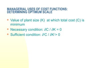

![(1) PROFIT CONTRIBUTION ANALYSIS
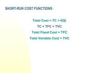
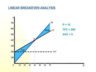
Total Revenue = TR = (P)(Q)
Total Cost = TC = TFC + (AVC)(Q)
Profit = TR -TC
Profit = Π = PQ - [TFC + (AVC)(Q)]
Q = TFC + Π
P - (AVC)
Profit contribution = P - AVC](https://image.slidesharecdn.com/f0dd9cost-130507023150-phpapp02/85/F0dd9-cost-34-320.jpg)

![(3) OPERATING LEVERAGE
Operating Leverage = TFC/TVC
Degree of Operating Leverage (or profit elasticity) = DOL
Π = PQ - TFC + (AVC)(Q)
= Q(P - AVC) - TFC
∆Π = ∆Q(P - AVC)
DOL = %∆Π = ∆Π/ Π = ∆Π * Q = E Π
%∆Q ∆Q/Q ∆Q Π
DOL = ∆Q(P - AVC)Q = Q(P - AVC)
∆Q[Q(P - AVC) - TFC] Q(P - AVC) - TFC](https://image.slidesharecdn.com/f0dd9cost-130507023150-phpapp02/85/F0dd9-cost-42-320.jpg)

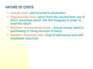
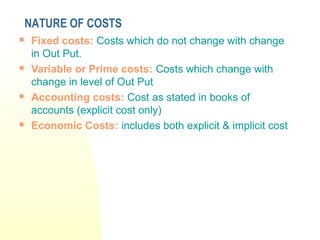
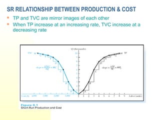
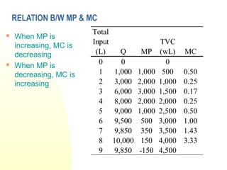
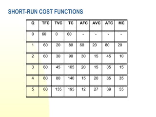
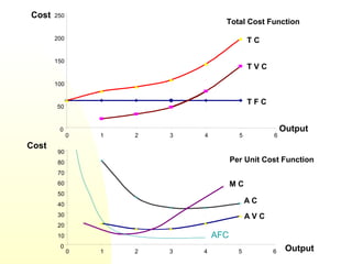
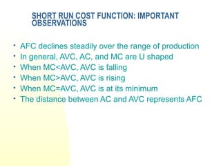
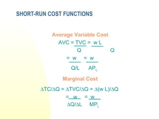
This document discusses various concepts related to cost theory and analysis. It defines different types of costs such as actual, opportunity, explicit, implicit, fixed, variable, accounting, economic, marginal, incremental, sunk, private, social, original, and replacement costs. It also discusses cost functions, the relationship between production and costs in the short-run and long-run, cost curves like total, average, and marginal costs. Finally, it covers special topics like profit contribution analysis, break-even analysis, operating leverage, learning curves, and economies of scope.