Downloaded 573 times

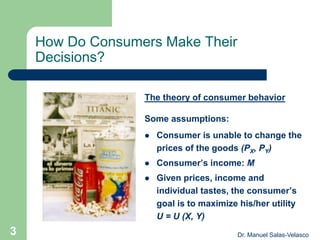
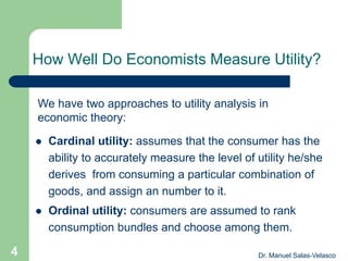


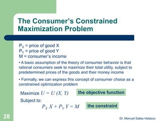
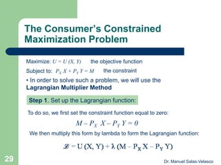
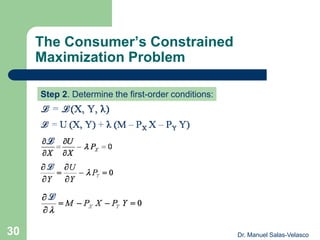
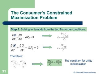
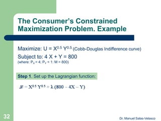
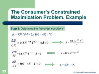
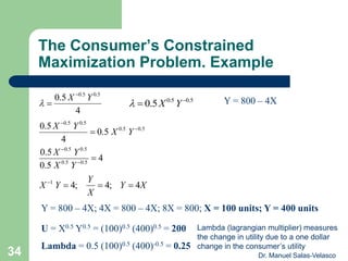
The document discusses consumer behavior in relation to utility and demand, introducing cardinal and ordinal utility concepts. It explains how consumers maximize utility given their income and the prices of goods, utilizing models like indifference curves and budget constraints. Additionally, it outlines the consumer's constrained maximization problem through the Lagrangian method, emphasizing the conditions for utility maximization.