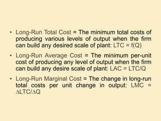
Downloaded 85 times


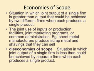
![Long-Run Cost Curves
• The long run is the period of time during which:
Technology is constant
All inputs and costs are variable
The firm faces no fixed inputs or costs
The long run period is a series of short run
periods. [For each short run period there is a
set of TP, AP, MP, MC, AFC, AVC, ATC, TC,
TVC & TFC for each possible scale of plant].](https://image.slidesharecdn.com/costfunction-130929214212-phpapp02/85/Cost-function-10-320.jpg)
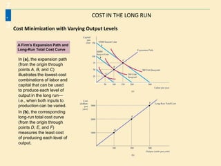
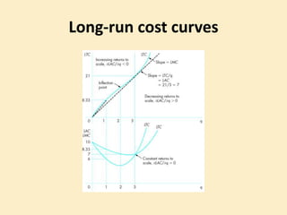
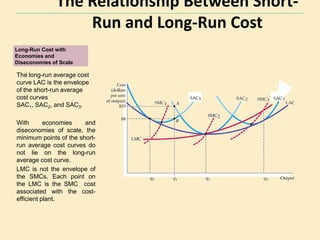
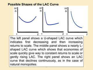
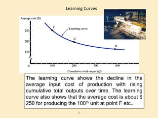

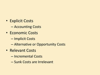
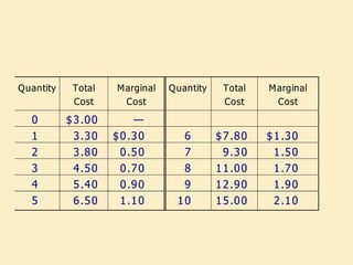
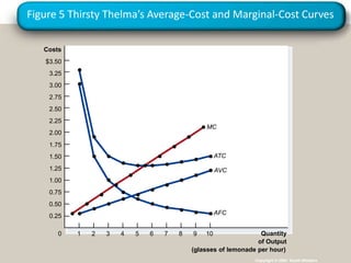
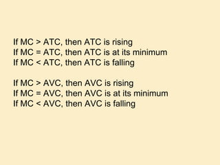
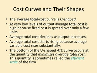
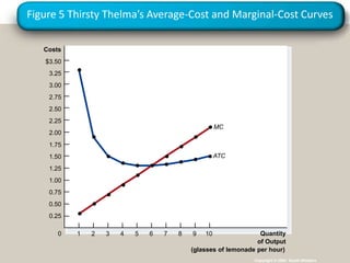
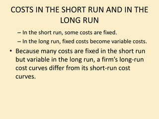
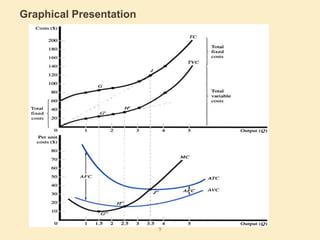
- The document discusses different types of costs including explicit, economic, and relevant costs. It also discusses short-run and long-run costs. - Graphs show cost curves including average total cost, average variable cost, marginal cost, and how they relate to quantity produced. - The shapes of long-run cost curves are explained, including how returns to scale impact the average cost curve. Economies and diseconomies of scale as well as learning curves are also summarized.


![6. Costs Management MEn BE me something in ibsbeMBA.pptxAutosaved].pptx](https://cdn.slidesharecdn.com/ss_thumbnails/6-251228180457-10e76ffe-thumbnail.jpg?width=640&height=640&fit=bounds)


![Dividends and _dividend_policy_powerpoint_presentation[1]](https://cdn.slidesharecdn.com/ss_thumbnails/dividendsanddividendpolicypowerpointpresentation1-130929215028-phpapp02-thumbnail.jpg?width=640&height=640&fit=bounds)


