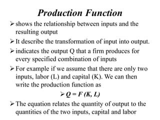
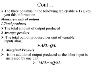
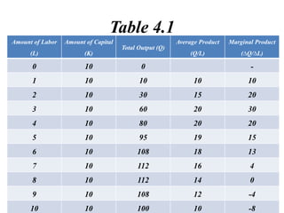
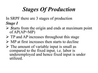
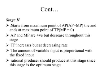
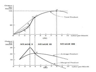
This document defines production and costs, and discusses the theory of production and cost. It covers: 1) Definitions of production, inputs, production functions, and the relationship between inputs and output. 2) The characteristics of short-run and long-run production periods and production functions. 3) The measurement of total product, average product, and marginal product and how they relate at different stages of production. 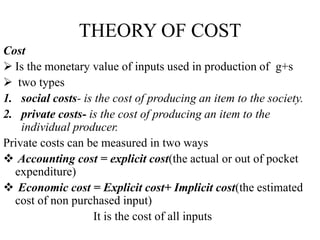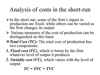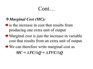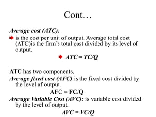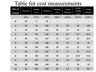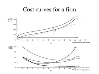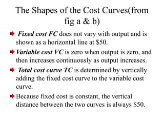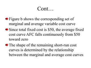4) Cost concepts including total, fixed, variable, marginal, average, and their relationships as depicted through cost curves.

1. CHAPTER FOUR
THEORY OF PRODUCTION AND
COST

2. Definition of Production and
Production Function
Production
 is the process of changing inputs into output
Is the process of using the services of inputs to
make g+s available.
Input
is anything that can be used in the production of
g+s. include labor, capital, land and
entrepreneurship.
There are two types of inputs

3. Cont….
Fixed inputs-inputs that cannot vary overtime
Or inputs whose quantity remain fixed for a
given period of time.
Example: machineries, capital
Variable inputs –those inputs whose quantity
vary overtime
• Example: labour

4. Production Function
shows the relationship between inputs and the
resulting output
It describe the transformation of input into output.
indicates the output Q that a firm produces for
every specified combination of inputs
For example if we assume that there are only two
inputs, labor (L) and capital (K). We can then
write the production function as
Q = F (K, L)
The equation relates the quantity of output to the
quantities of the two inputs, capital and labor

5. Production period
The Short run vs Long run period
Showing the nature of economic adjustment in the
firm to changing economic environment.
Short run
refers to a period of time in which at least one
input remain fixed.
Long run
refers to a period of time in which all factors of
production are variable

6. The Short run Production Function
The production function is said to short run if there
exist at least one fixed input in the production.
In this case it is assumed that there is only one
variable input
 This variable input is usually called “labor”
 It is also assumed that this variable input can be
combined in different proportions with the fixed
variable input to produce various quantities of
output.

7. Cont…
Consider the case in which capital is fixed, but
labor is variable, so that the firm can produce
more output by increasing its labor input
 Imagine, for example, that you are managing a
clothing plant
 You have to decide how much labor to hire and
how much clothing to produce
To make the decision, you will need to know how
the amount of output Q increases (if at all), as the
input of labor L increases

8. Cont…
The three columns in the following table(table 4.1) gives
you this information
Measurements of output
1.Total products
The total amount of output produced
2.Average product
 The total output produced per unit of variable
input(labor)
APL=Q/L
3. Marginal Product
 is the additional output produced as the labor input is
increased by one unit
 MPL= ∆Q/∆L

9. Table 4.1
Amount of Labor
(L)
Amount of Capital
(K)
Total Output (Q)
Average Product
(Q/L)
Marginal Product
(∆Q/∆L)
0 10 0 -
1 10 10 10 10
2 10 30 15 20
3 10 60 20 30
4 10 80 20 20
5 10 95 19 15
6 10 108 18 13
7 10 112 16 4
8 10 112 14 0
9 10 108 12 -4
10 10 100 10 -8

10. Stages Of Production
In SRPF there are 3 stages of production
Stage I
 Starts from the origin and ends at maximum point
of AP(AP=MP)
 TP and AP increases throughout this stage
 MP at first increases then starts to decline
 The amount of variable input is small as
compared to the fixed input. i.e. labor is
underemployed and hence fixed input is under
utilized.

11. Cont…
Stage II
 Starts from maximum point of AP(AP=MP) the and
ends at maximum point of TP(MP = 0)
 AP and MP are +ve but decrease throughout this
stage
 TP increases but at decreasing rate
 The amount of variable input is proportional with
the fixed input
 rational producer should produce at this stage since
this stage is the optimum stage.

12. Cont…
Stage III
 Starts from the maximum point of TP and
endless(whenever MP is negative)
 TP and AP decreases throughout this stage
 MP decreases and even negative
 The amount of variable input is greater as compared to
the fixed input
 Each additional unit of labor contributing negatively to
total product due to excess of variable input over fixed
input. i.e. over utilization due to over
employment….due to this, this stage also known as
extensive margin.

13. Graphically

14. The law of diminishing marginal
returns
• The law states that as increasing amount of
variable input is combines with fixed inputs,
eventually the contribution of each additional
amount of the variable input to the TP
declines.
• The law starts to operate after the MP curve
reaches its maximum.

15. Cont…..
• When total product is maximum, marginal
product is zero
• When Mp equals AP, AP reaches its maximum.
• whenever, MP of the variable input is less
than AP, the AP decreases.
• Whenever MP>AP, AP increases

16. Production function with two variable
input
• When Labor and capital are variable input…long run
production
• Given two variable input one can produce the same
level of product by different combination of those two
input.
• A table that represent the various combination of
labor and capital which give the producer the same
level of output is called isoquant schedule or equal
product schedule.

17. isoquant schedule or equal product
schedule.
Combination Capital Labor Maximum
output
MRTs of capital
for labor
A 1 11 60 -
B 2 7 60 4:1
C 3 4 60 3:1
D 4 2 60 2:1
E 5 1 60 1:1

18. • A graphical representation of isoquant
schedule is called iso product curve or equal
product curve or simply isoquant.
• Isoquant refers to those combination ot two
variable inputs that yields the same level of
output. k
labor

19. Cont…
• Isoquant map is the set of isoquant or equal
product curves.
• Each successive isoquant to the right represents
higher level of total product because it reflect the
use of more of at least one of the two input.
Properties of isoquant
1. Isoquant slopes downward
2. It is concave to the origin……MRTS
3. Isoquant never cross each other

20. The economic region of production
• the the region in which the producer should
produce in case of two variable input like in
the case of stage II for short run prodction.
• Implying that the producer should select
those combinations that may not employee
him/her more of labor or capital

21. Marginal rate of technical substitution
(MRTS)
• Shows an entrepreneurs willingness to substitute one
input by another input so as to be efficient in
production.
• The rate at which one input is substituted by another
input to get the same level of output is called MRTS.
• MRTS = ∆L/∆K
• (See the previous example)….show that the
principle of diminshing marginal rate of technical
substitution, determining the shape of the isoquant

22. Return to scale
• Is a property of production function that indicate the
relationship between proportionate change in all inputs
and the resulting change in total product.
• It is a property that apply only in the long run.
• Three types
1. constant return to scale:- %∆ in all input = %∆in output
2. Increasing return to scale:- %∆ in all input < %∆in outpt
3. Decreasing return to scale :- %∆ in all i/pt > %∆in outpt

23. Increasing return to scale may occur
because of:
a. An increase in the scale of operation…using specialized
machinery
b. Greater division of labor
c. Greater degree of specialization
effect of technological change on production function
• Technological advancement makes our limited resource
more productive.
• More output from the existing level of inputs
• The existing level of output by using less of the inputs
• It shift the TP curve up(isoquant curve down) implying
that we can produce more of the product than before.

24. THEORY OF COST
Cost
 Is the monetary value of inputs used in production of g+s
 two types
1. social costs- is the cost of producing an item to the society.
2. private costs- is the cost of producing an item to the
individual producer.
Private costs can be measured in two ways
 Accounting cost = explicit cost(the actual or out of pocket
expenditure)
 Economic cost = Explicit cost+ Implicit cost(the estimated
cost of non purchased input)
It is the cost of all inputs

25. Analysis of costs in the short-run
In the short run, some of the firm’s inputs to
production are fixed, while others can be varied as
the firm changes its output
 Various measures of the cost of production can be
distinguished on this basis
Total Cost (TC): The total cost of production has
two components:
1. Fixed cost (FC), which is borne by the firm
whatever level of output it produces
2. Variable cost (VC), which varies with the level of
output
TC = TFC + TVC

26. Cont…
Marginal Cost (MC):
is the increase in cost that results from
producing one extra unit of output
Marginal cost is just the increase in variable
cost that results from an extra unit of output.
We can therefore write marginal cost as
MC = ∆TC/∆Q = ∆TVC/∆Q

27. Cont…
Average cost (ATC):
is the cost per unit of output. Average total cost
(ATC)is the firm’s total cost divided by its level of
output.
ATC = TC/Q
ATC has two components.
Average fixed cost (AFC) is the fixed cost divided by
the level of output.
AFC = FC/Q
Average Variable Cost (AVC): is variable cost divided
by the level of output.
AVC = VC/Q

28. Table for cost measurements
Rate of
Output
Fixed Cost
Variable
Cost
Total Cost
Marginal
Cost
Average
Fixed Cost
Average
Variable
Cost
Average
Total Cost
(FC) (VC) (TC) (MC) (AFC) (AVC) (ATC)
0 50 0 50 - - - -
1 50 50 100 50 50 50 100
2 50 78 128 28 25 39 64
3 50 98 148 20 16.7 32.7 49.3
4 50 112 162 14 12.5 28 40.5
5 50 130 180 18 10 26 36
6 50 150 200 20 8.3 25 33.3
7 50 175 225 25 7.1 25 32.1
8 50 204 254 29 6.3 25.5 31.8
9 50 242 292 38 5.6 26.9 32.4
10 50 300 350 58 5 30 35
11 50 385 435 85 4.5 35 39.5

29. Cost curves for a firm

30. The Shapes of the Cost Curves(from
fig a & b)
Fixed cost FC does not vary with output and is
shown as a horizontal line at $50.
Variable cost VC is zero when output is zero, and
then increases continuously as output increases.
Total cost curve TC is determined by vertically
adding the fixed cost curve to the variable cost
curve.
Because fixed cost is constant, the vertical
distance between the two curves is always $50.

31. Cont…
Figure b shows the corresponding set of
marginal and average variable cost curve
Since total fixed cost is $50, the average fixed
cost curve AFC falls continuously from $50
toward zero
The shape of the remaining short-run cost
curves is determined by the relationship
between the marginal and average cost curves

32. Cont…
Whenever marginal cost lies below average
cost,(MC<AC) the average cost curve falls.
Whenever marginal cost lies above average
cost,(MC>AC) the average cost curve rises. And
when average cost is at a minimum, marginal cost
equals average cost
The ATC curve shows the average total cost of
production
The vertical distance between the ATC and AVC
curves decreases as output increases

33. Cont…
The AVC cost curve achieves its minimum point
at a lower output than the ATC curve
This follows because MC = AVC at its minimum
point, and MC = ATC at its minimum point.
Since ATC is always greater than AVC and the
marginal cost curve MC is rising, the minimum
point of the ATC curve must lie above and to the
right of the minimum point of the AVC curve.