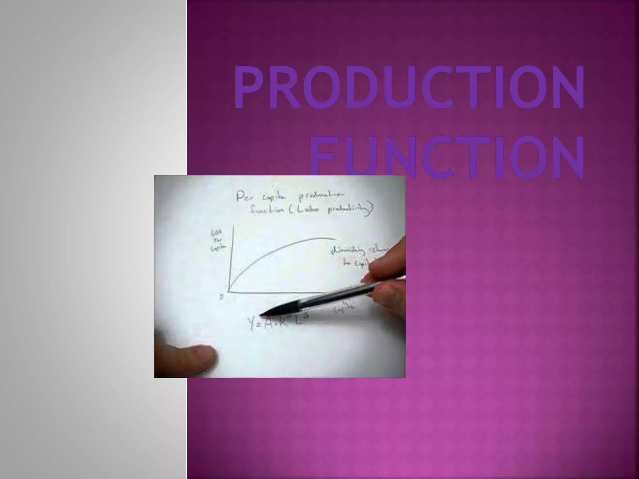
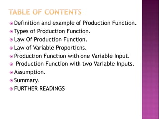
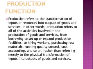
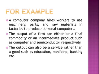
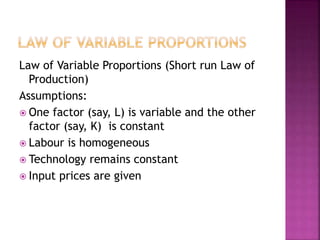
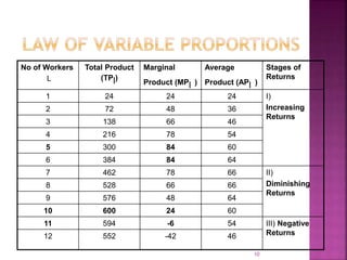
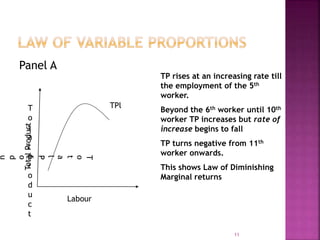
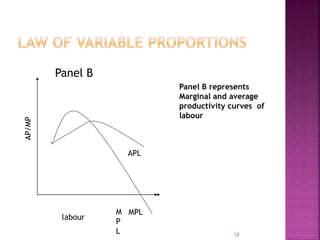
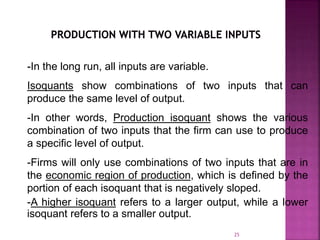
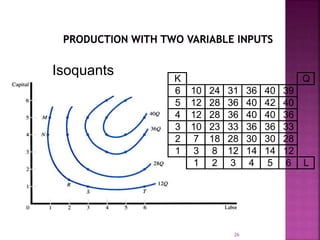
 Definition and example of Production Function.
 Types of Production Function.
 Law Of Production Function.
 Law of Variable Proportions.
 Production Function with one Variable Input.
 Production Function with two Variable Inputs.
 Assumption.
 Summary.
 FURTHER READINGS
 Production refers to the transformation of
inputs or resources into outputs of goods and
services. In other words, production refers to
all of the activities involved in the
production of goods and services, from
borrowing to set up or expand production
facilities, to hiring workers, purchasing row
materials, running quality control, cost
accounting, and so on, rather than referring
merely to the physical transformation of
inputs into outputs of goods and services.
 A computer company hires workers to use
machinery, parts, and raw materials in
factories to produce personal computers.
 The output of a firm can either be a final
commodity or an intermediate product such
as computer and semiconductor respectively.
 The output can also be a service rather than
a good such as education, medicine, banking
etc.
 Mathematical representation of the relationship:
 Q = f (K, L, La)
 Output (Q) is dependent upon the amount of capital
(K), Land(L) and Labour (La) used
 There are two distinct types of production
function that show possible range of
substitution inputs in the production process.
 1. Fixed proportion Production function
 2. Variable proportions production function
Short term : Time when one input (say,
capital) remains constant and an addition to
output can be obtained only by using more
labour.
Long run: Both inputs become variable.
Production process is
subject to various
phases-
Laws of production state the relationship
between output and input.
Short run :
Relationship between input and output are studied
by varying one input , others being held
constant.
Law of Variable Proportions brings out
relationship between varying proportions of
factor inputs and output
Long run:
Production function is subject to different phases
described under the Law of Returns to Scale
– Studied assuming that all factor inputs are
variable.
Law of Variable Proportions (Short run Law of
Production)
Assumptions:
 One factor (say, L) is variable and the other
factor (say, K) is constant
 Labour is homogeneous
 Technology remains constant
 Input prices are given
No of Workers
L
Total Product
(TPl)
Marginal
Product (MPl )
Average
Product (APl )
Stages of
Returns
1 24 24 24 I)
Increasing
Returns
2 72 48 36
3 138 66 46
4 216 78 54
5 300 84 60
6 384 84 64
7 462 78 66 II)
Diminishing
Returns
8 528 66 66
9 576 48 64
10 600 24 60
11 594 -6 54 III) Negative
Returns
12 552 -42 46
10
Panel A
11
Labour
T
o
t
a
l
p
r
o
d
u
c
t
T
o
t
a
l
P
r
o
d
u
Total
Product
TPl
TP rises at an increasing rate till
the employment of the 5th
worker.
Beyond the 6th worker until 10th
worker TP increases but rate of
increase begins to fall
TP turns negative from 11th
worker onwards.
This shows Law of Diminishing
Marginal returns
Panel B
12
labour
APL
M
P
L
MPL
Panel B represents
Marginal and average
productivity curves of
labour
AP/MP
Increasing Returns- Stage I:
TPl increases at an increasing rate.
Fixed factor (K) is abundant and variable factor is
inadequate. Hence K gets utilized better with
every additional unit of labour
Stage II- TPl continues to increase but at a
diminishing rate.
stage III- TPl begins to decline –Capital becomes
scarce as compared to variable factor. Hence over
utilization of capital and setting in of diminishing
returns
Causes of 3 stages: Indivisibility and inelasticity of
fixed factor and imperfect substitutability between
K and L
13
Significance of Law of Diminishing Marginal
Returns:
- Empirical law, frequently observed in various
production activities
- Particularly in agriculture where natural
factors (say land), which play an important
role, are limited.
- Helps manager in identifying rational and
irrational stages of operation
14
- It provides answers to questions such as:
a) How much to produce?
b) What number of workers (and other
variable factors) to employ in order to
maximize output
In our example, firm should employ a minimum
of 7 workers and maximum of 10 workers
(where TP is still rising)
15
- Stage III has very high L-K ratio- as a result,
additional workers not only prove
unproductive but also cause a decline in TPl.
- In Stage I capital is presumably under-
utilised.
- So a firm operating in Stage I has to increase
L and that in Stage III has to decrease labour.
16
 There are two Variable Proportions
Production
Function_
1- Production Function With One Variable
Input.
2- Production With Two Variable Inputs
18
 When discussing production in the short
run, three definitions are important:
 Total product
 Marginal product
 Average product
19
Total Product
Marginal Product
Average Product
Production or
Output Elasticity
TP = Q = f(L)
MPL =
TP
L
APL =
TP
L
EL =
MPL
APL
20
Total Product
 Total product (TP) is another name for output
in the short run.
TP = Q = f (L)
21
 The marginal product (MP) of a variable
input is the change in output (or TP)
resulting from a one unit change in the
input.
 MP tells us how output changes as we
change the level of the input by one unit.
 Consider the two input production function
Q=f (L,K) in which input L is variable and
input K is fixed at some level.
 The marginal product of input L is defined
as holding input K constant.
MPL =
TP
L
22
 The average product (AP) of an input is the
total product divided by the level of the
input.
 AP tells us, on average, how many units of
output are produced per unit of input used.
 The average product of input L is defined
as holding input K constant.
APL =
TP
L
23
L Q MPL APL EL
0 0 - - -
1 3 3 3 1
2 8 5 4 1.25
3 12 4 4 1
4 14 2 3.5 0.57
5 14 0 2.8 0
6 12 -2 2 -1
Total, Marginal, and Average Product of Labor, and Output Elasticity
24
25
-In the long run, all inputs are variable.
Isoquants show combinations of two inputs that can
produce the same level of output.
-In other words, Production isoquant shows the various
combination of two inputs that the firm can use to produce
a specific level of output.
-Firms will only use combinations of two inputs that are in
the economic region of production, which is defined by the
portion of each isoquant that is negatively sloped.
-A higher isoquant refers to a larger output, while a lower
isoquant refers to a smaller output.
26
Isoquants K Q
6 10 24 31 36 40 39
5 12 28 36 40 42 40
4 12 28 36 40 40 36
3 10 23 33 36 36 33
2 7 18 28 30 30 28
1 3 8 12 14 14 12
1 2 3 4 5 6 L
 THE PRODUCTION FUNCTIONS ARE BASED ON
CERTAIN ASSUMPTIONS.
 1 Perfect divisibility of both inputs and outputs
 2 Limited substitution of one factor for another
 3 Constant technology
 4 Inelastic supply of fixed factors in
the short run
 A production function specifies the maximum
output that can be produced with
 a given set of inputs. In order to achieve
maximum profits the production
 manager has to use optimum input-output
combination for a given cost. In this
 unit, we have shown how a production
manager minimizes the cost for a given
 output in order to maximize the profit. Also,
we have shown how to maximize
 the output at a given level of cost.
 Adhikary, M (1987), Managerial Economics
(Chapter V), Khosla,Publishing House, Delhi.
 Google.
Economics for decision Making

Economics for decision Making

  • 2.
     Definition andexample of Production Function.  Types of Production Function.  Law Of Production Function.  Law of Variable Proportions.  Production Function with one Variable Input.  Production Function with two Variable Inputs.  Assumption.  Summary.  FURTHER READINGS
  • 3.
     Production refersto the transformation of inputs or resources into outputs of goods and services. In other words, production refers to all of the activities involved in the production of goods and services, from borrowing to set up or expand production facilities, to hiring workers, purchasing row materials, running quality control, cost accounting, and so on, rather than referring merely to the physical transformation of inputs into outputs of goods and services.
  • 4.
     A computercompany hires workers to use machinery, parts, and raw materials in factories to produce personal computers.  The output of a firm can either be a final commodity or an intermediate product such as computer and semiconductor respectively.  The output can also be a service rather than a good such as education, medicine, banking etc.
  • 5.
     Mathematical representationof the relationship:  Q = f (K, L, La)  Output (Q) is dependent upon the amount of capital (K), Land(L) and Labour (La) used
  • 6.
     There aretwo distinct types of production function that show possible range of substitution inputs in the production process.  1. Fixed proportion Production function  2. Variable proportions production function
  • 7.
    Short term :Time when one input (say, capital) remains constant and an addition to output can be obtained only by using more labour. Long run: Both inputs become variable. Production process is subject to various phases- Laws of production state the relationship between output and input.
  • 8.
    Short run : Relationshipbetween input and output are studied by varying one input , others being held constant. Law of Variable Proportions brings out relationship between varying proportions of factor inputs and output Long run: Production function is subject to different phases described under the Law of Returns to Scale – Studied assuming that all factor inputs are variable.
  • 9.
    Law of VariableProportions (Short run Law of Production) Assumptions:  One factor (say, L) is variable and the other factor (say, K) is constant  Labour is homogeneous  Technology remains constant  Input prices are given
  • 10.
    No of Workers L TotalProduct (TPl) Marginal Product (MPl ) Average Product (APl ) Stages of Returns 1 24 24 24 I) Increasing Returns 2 72 48 36 3 138 66 46 4 216 78 54 5 300 84 60 6 384 84 64 7 462 78 66 II) Diminishing Returns 8 528 66 66 9 576 48 64 10 600 24 60 11 594 -6 54 III) Negative Returns 12 552 -42 46 10
  • 11.
    Panel A 11 Labour T o t a l p r o d u c t T o t a l P r o d u Total Product TPl TP risesat an increasing rate till the employment of the 5th worker. Beyond the 6th worker until 10th worker TP increases but rate of increase begins to fall TP turns negative from 11th worker onwards. This shows Law of Diminishing Marginal returns
  • 12.
    Panel B 12 labour APL M P L MPL Panel Brepresents Marginal and average productivity curves of labour AP/MP
  • 13.
    Increasing Returns- StageI: TPl increases at an increasing rate. Fixed factor (K) is abundant and variable factor is inadequate. Hence K gets utilized better with every additional unit of labour Stage II- TPl continues to increase but at a diminishing rate. stage III- TPl begins to decline –Capital becomes scarce as compared to variable factor. Hence over utilization of capital and setting in of diminishing returns Causes of 3 stages: Indivisibility and inelasticity of fixed factor and imperfect substitutability between K and L 13
  • 14.
    Significance of Lawof Diminishing Marginal Returns: - Empirical law, frequently observed in various production activities - Particularly in agriculture where natural factors (say land), which play an important role, are limited. - Helps manager in identifying rational and irrational stages of operation 14
  • 15.
    - It providesanswers to questions such as: a) How much to produce? b) What number of workers (and other variable factors) to employ in order to maximize output In our example, firm should employ a minimum of 7 workers and maximum of 10 workers (where TP is still rising) 15
  • 16.
    - Stage IIIhas very high L-K ratio- as a result, additional workers not only prove unproductive but also cause a decline in TPl. - In Stage I capital is presumably under- utilised. - So a firm operating in Stage I has to increase L and that in Stage III has to decrease labour. 16
  • 17.
     There aretwo Variable Proportions Production Function_ 1- Production Function With One Variable Input. 2- Production With Two Variable Inputs
  • 18.
    18  When discussingproduction in the short run, three definitions are important:  Total product  Marginal product  Average product
  • 19.
    19 Total Product Marginal Product AverageProduct Production or Output Elasticity TP = Q = f(L) MPL = TP L APL = TP L EL = MPL APL
  • 20.
    20 Total Product  Totalproduct (TP) is another name for output in the short run. TP = Q = f (L)
  • 21.
    21  The marginalproduct (MP) of a variable input is the change in output (or TP) resulting from a one unit change in the input.  MP tells us how output changes as we change the level of the input by one unit.  Consider the two input production function Q=f (L,K) in which input L is variable and input K is fixed at some level.  The marginal product of input L is defined as holding input K constant. MPL = TP L
  • 22.
    22  The averageproduct (AP) of an input is the total product divided by the level of the input.  AP tells us, on average, how many units of output are produced per unit of input used.  The average product of input L is defined as holding input K constant. APL = TP L
  • 23.
    23 L Q MPLAPL EL 0 0 - - - 1 3 3 3 1 2 8 5 4 1.25 3 12 4 4 1 4 14 2 3.5 0.57 5 14 0 2.8 0 6 12 -2 2 -1 Total, Marginal, and Average Product of Labor, and Output Elasticity
  • 24.
  • 25.
    25 -In the longrun, all inputs are variable. Isoquants show combinations of two inputs that can produce the same level of output. -In other words, Production isoquant shows the various combination of two inputs that the firm can use to produce a specific level of output. -Firms will only use combinations of two inputs that are in the economic region of production, which is defined by the portion of each isoquant that is negatively sloped. -A higher isoquant refers to a larger output, while a lower isoquant refers to a smaller output.
  • 26.
    26 Isoquants K Q 610 24 31 36 40 39 5 12 28 36 40 42 40 4 12 28 36 40 40 36 3 10 23 33 36 36 33 2 7 18 28 30 30 28 1 3 8 12 14 14 12 1 2 3 4 5 6 L
  • 27.
     THE PRODUCTIONFUNCTIONS ARE BASED ON CERTAIN ASSUMPTIONS.  1 Perfect divisibility of both inputs and outputs  2 Limited substitution of one factor for another  3 Constant technology  4 Inelastic supply of fixed factors in the short run
  • 28.
     A productionfunction specifies the maximum output that can be produced with  a given set of inputs. In order to achieve maximum profits the production  manager has to use optimum input-output combination for a given cost. In this  unit, we have shown how a production manager minimizes the cost for a given  output in order to maximize the profit. Also, we have shown how to maximize  the output at a given level of cost.
  • 29.
     Adhikary, M(1987), Managerial Economics (Chapter V), Khosla,Publishing House, Delhi.  Google.