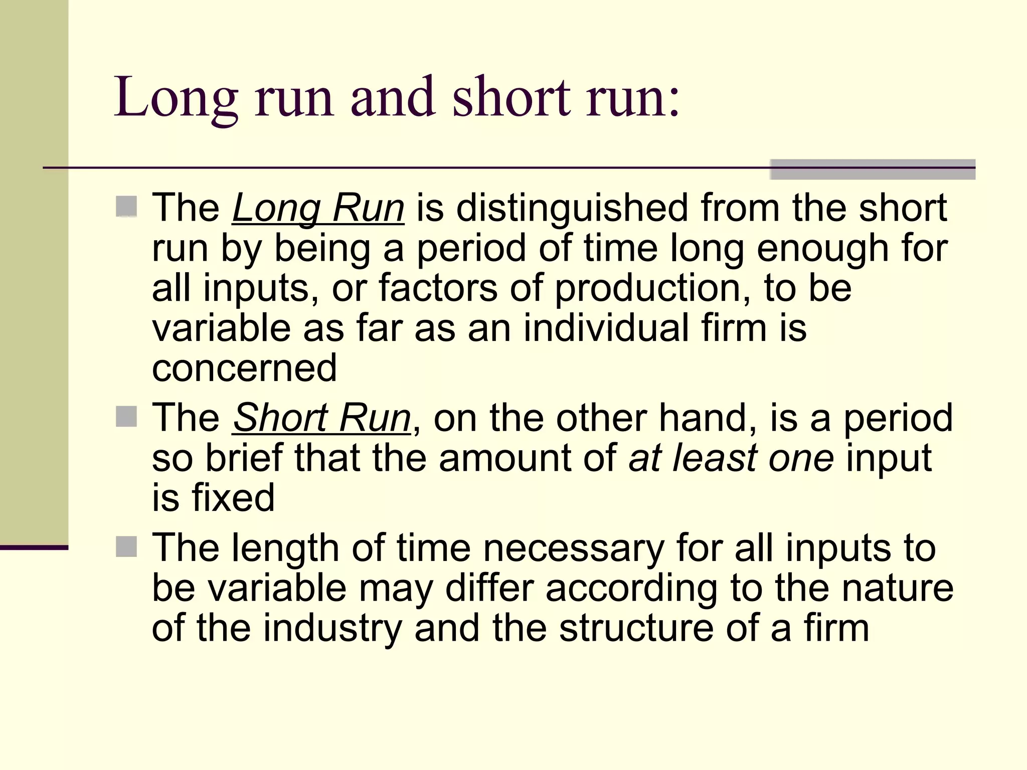
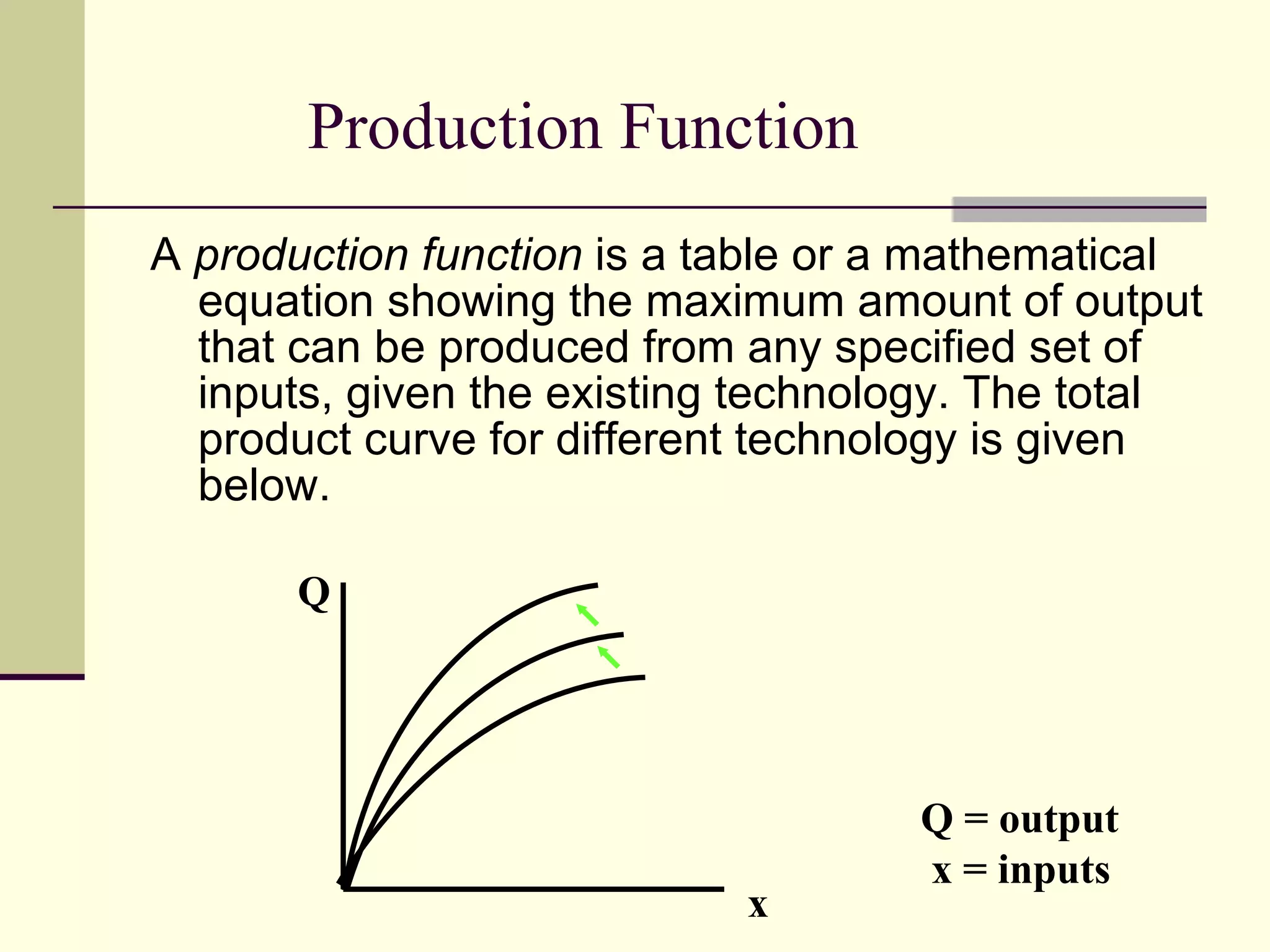
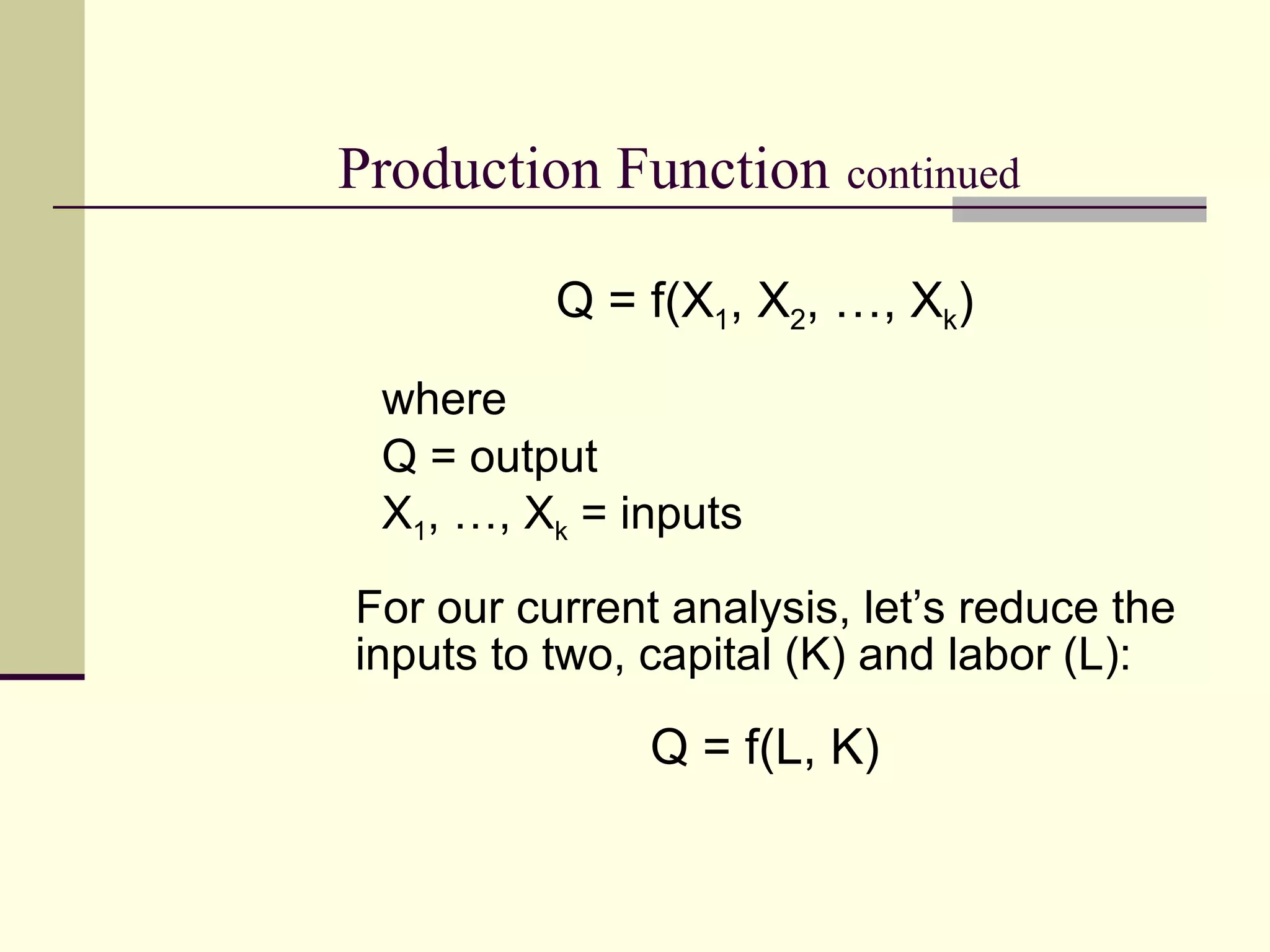
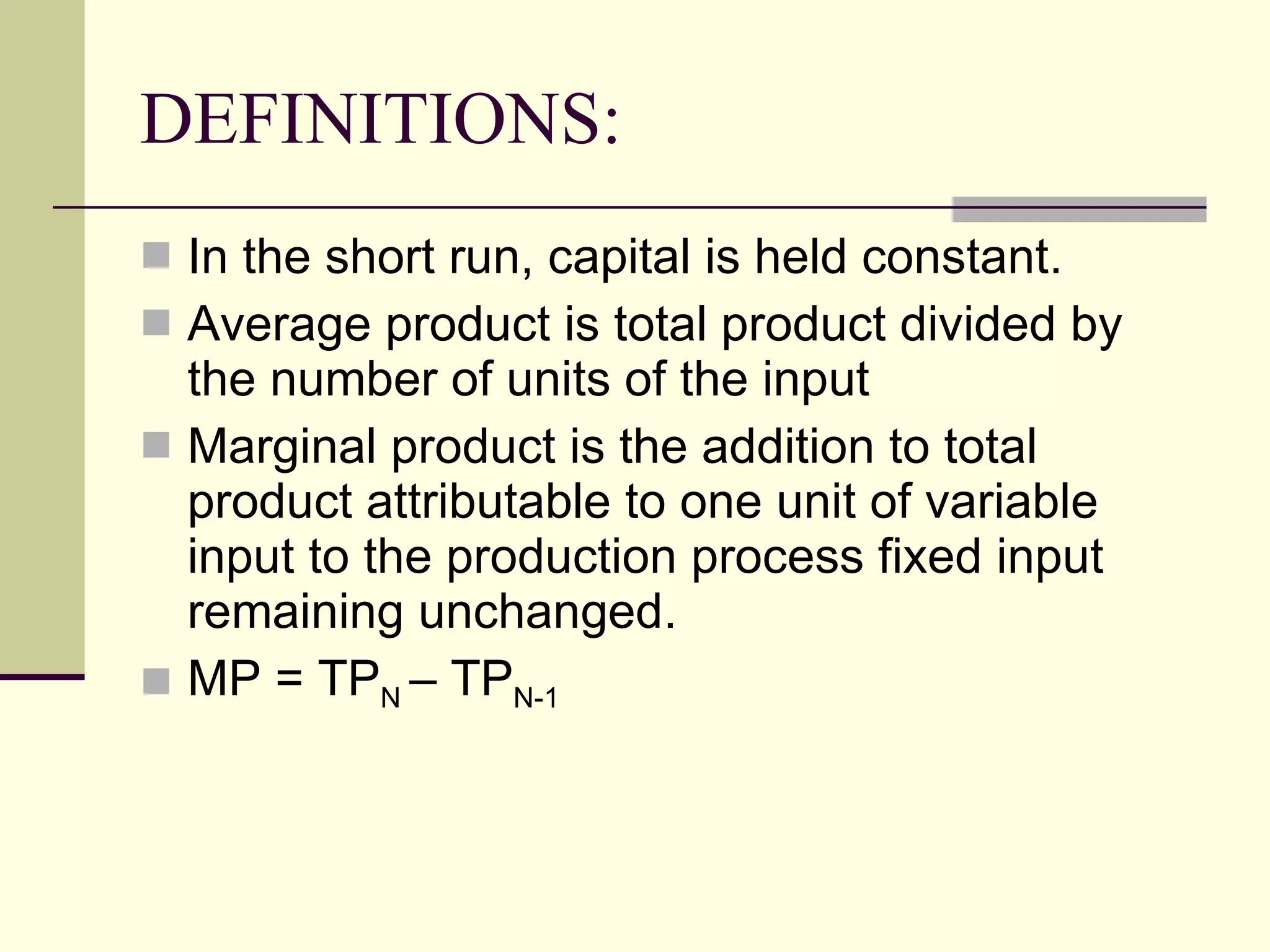
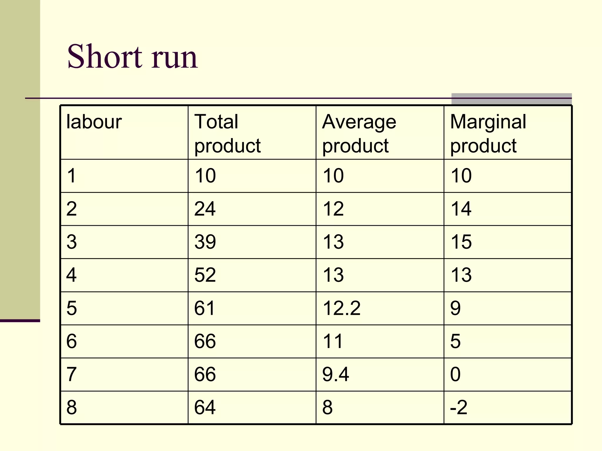
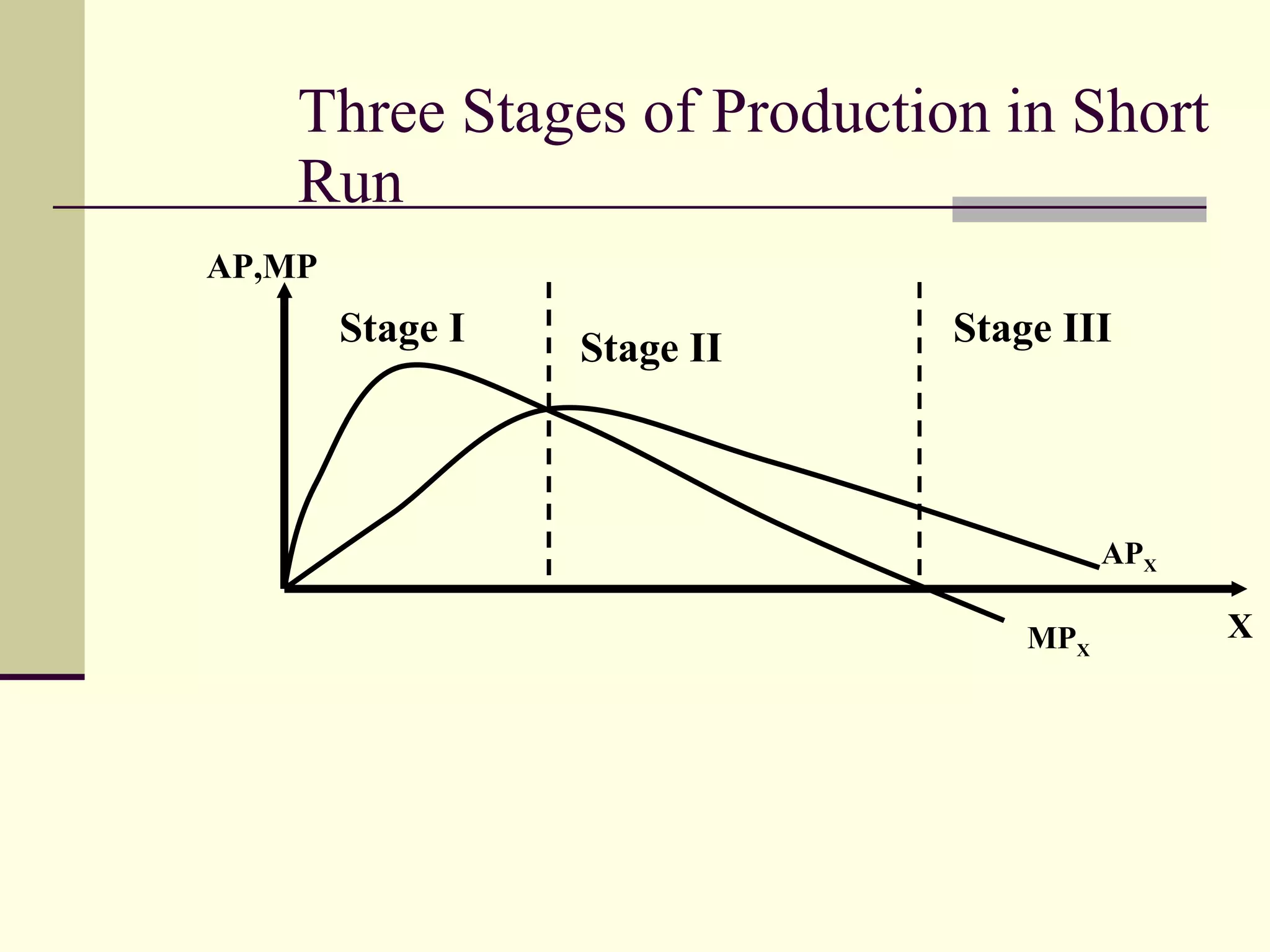
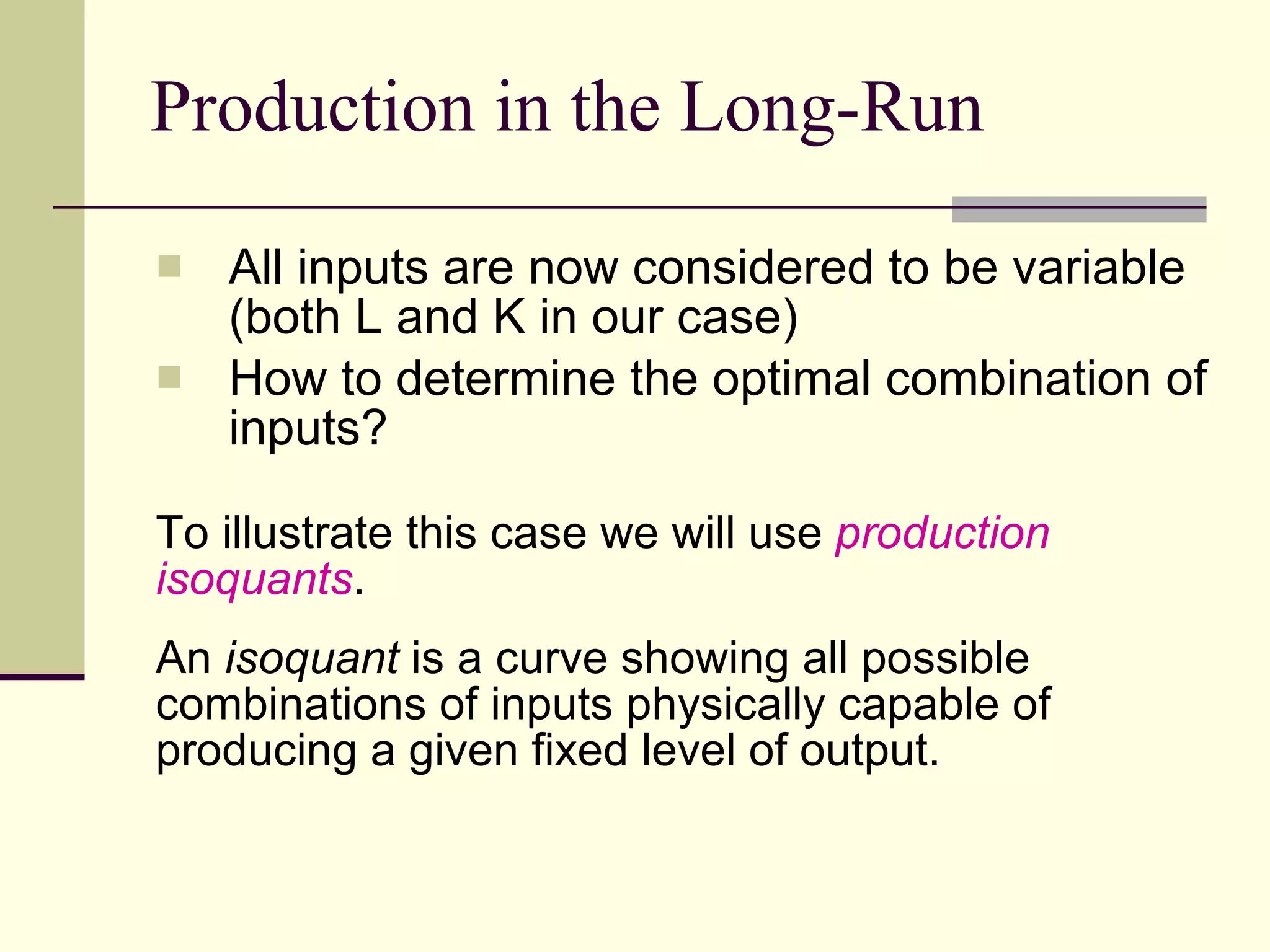
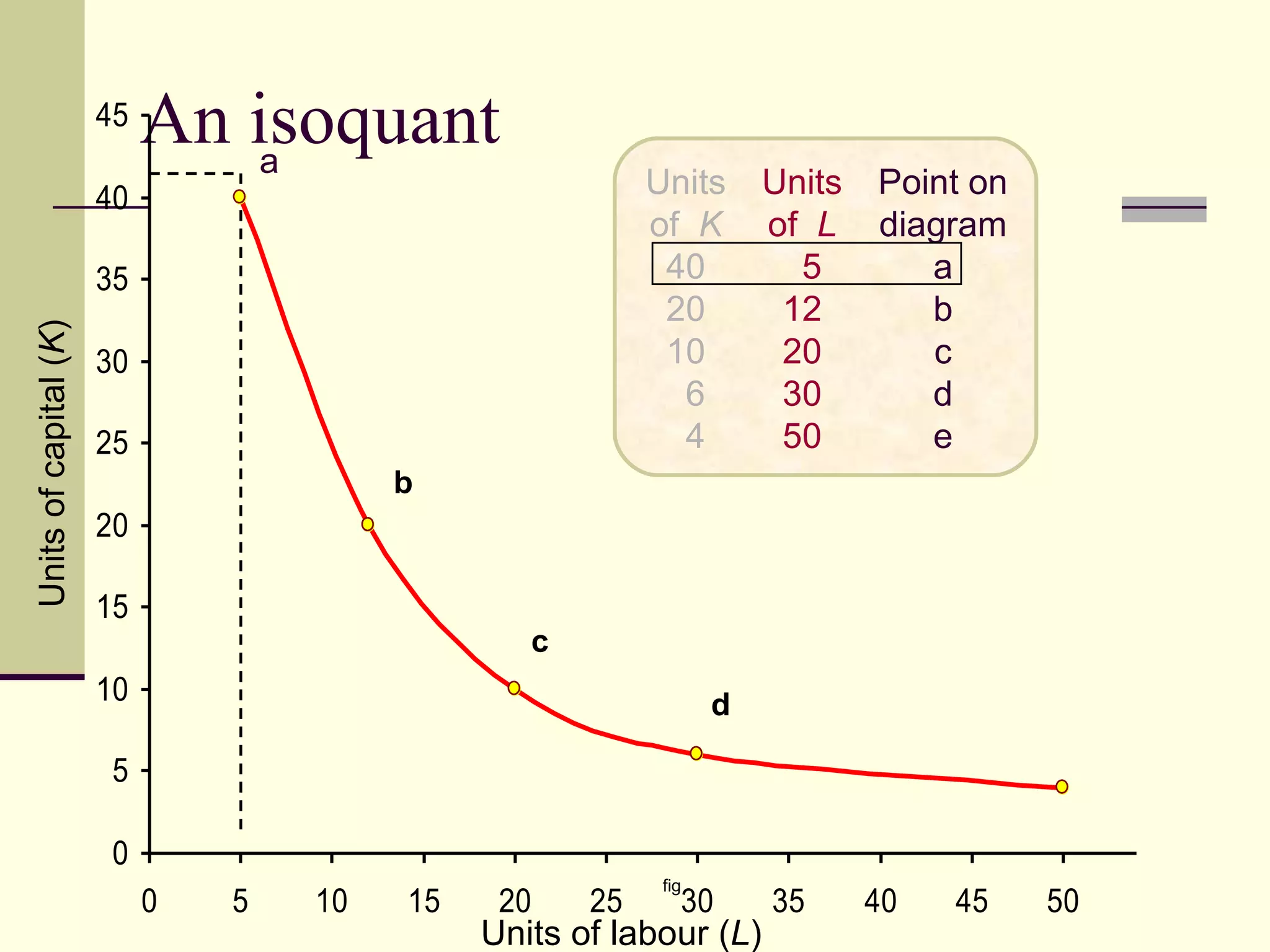
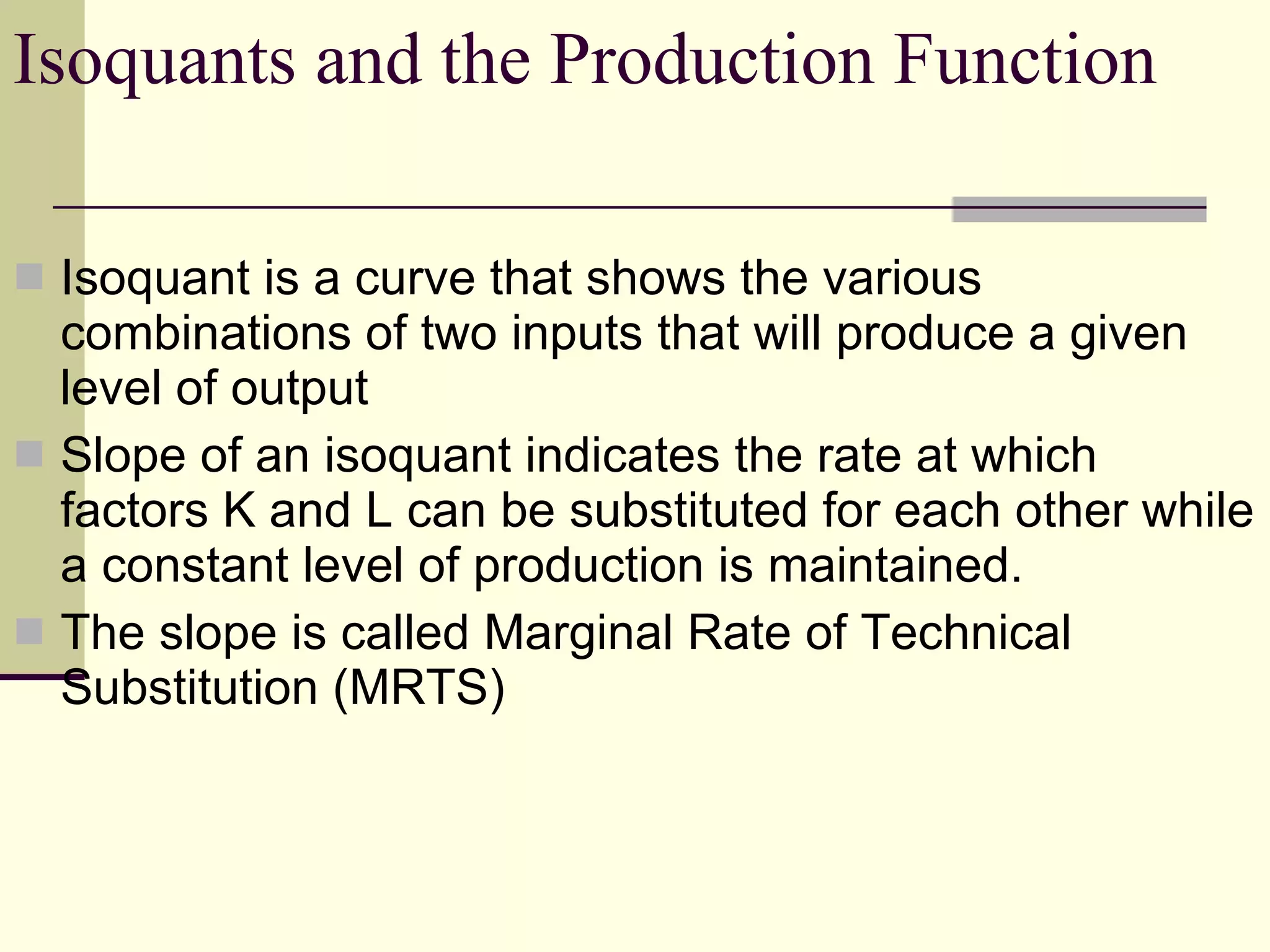
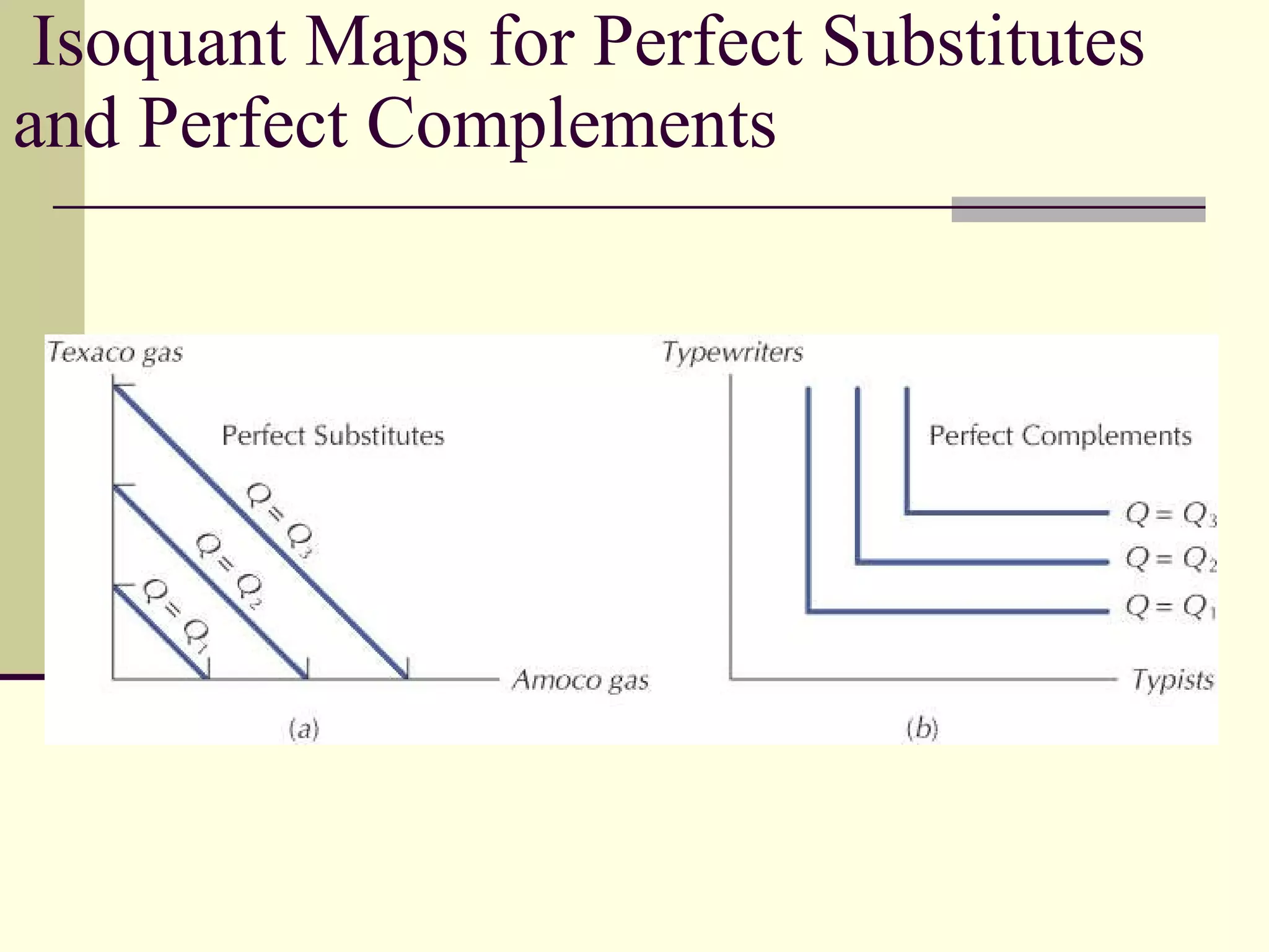
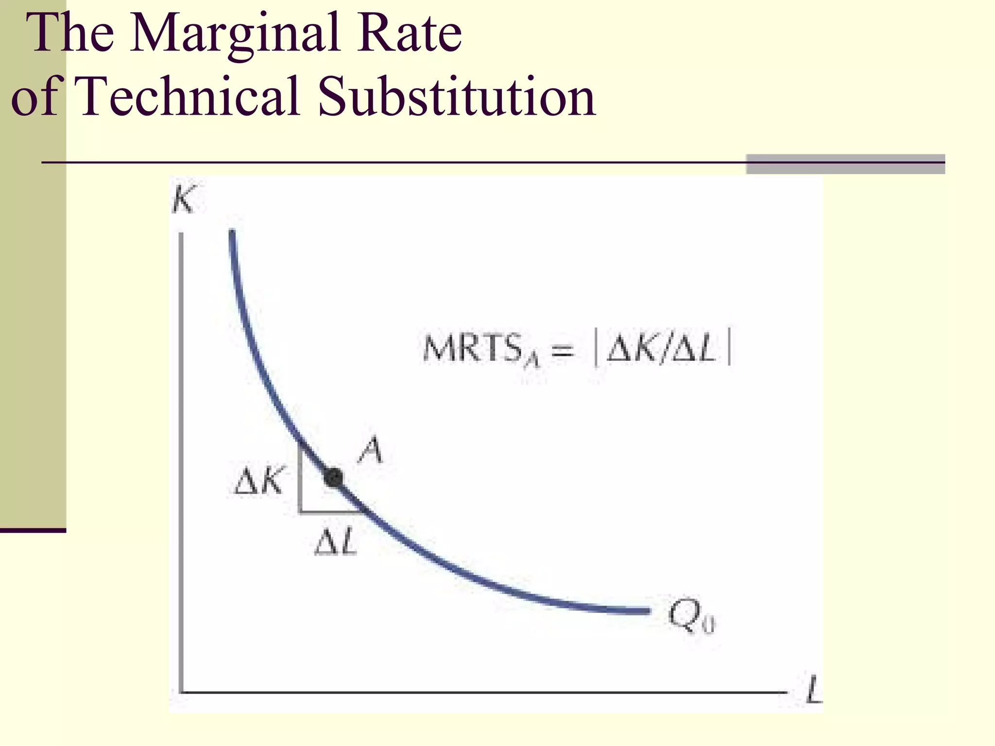
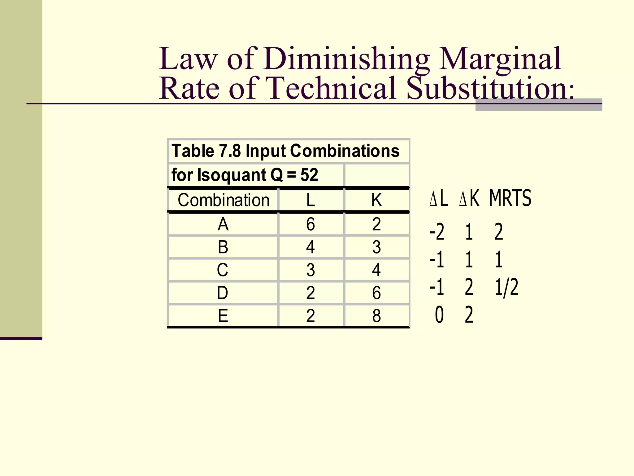
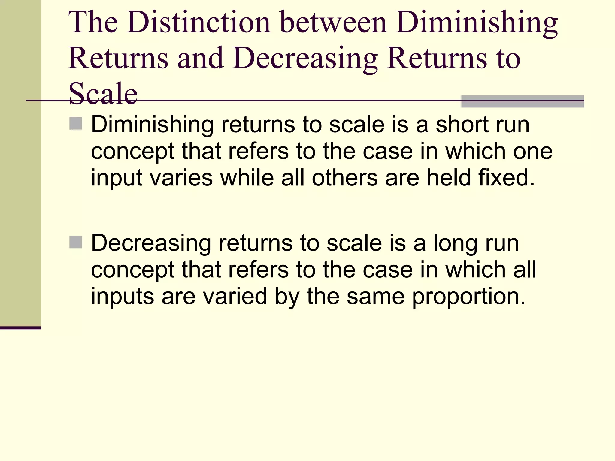
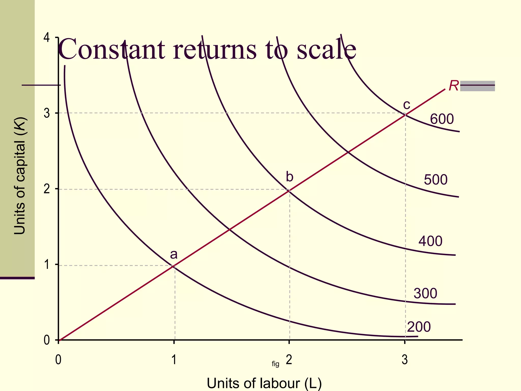
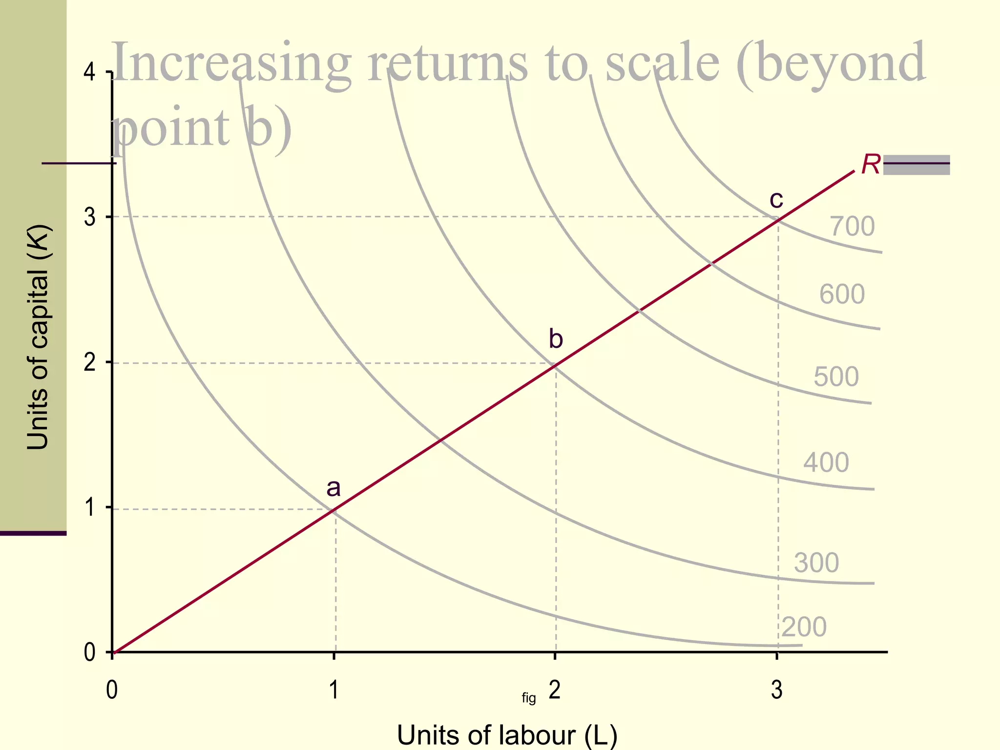
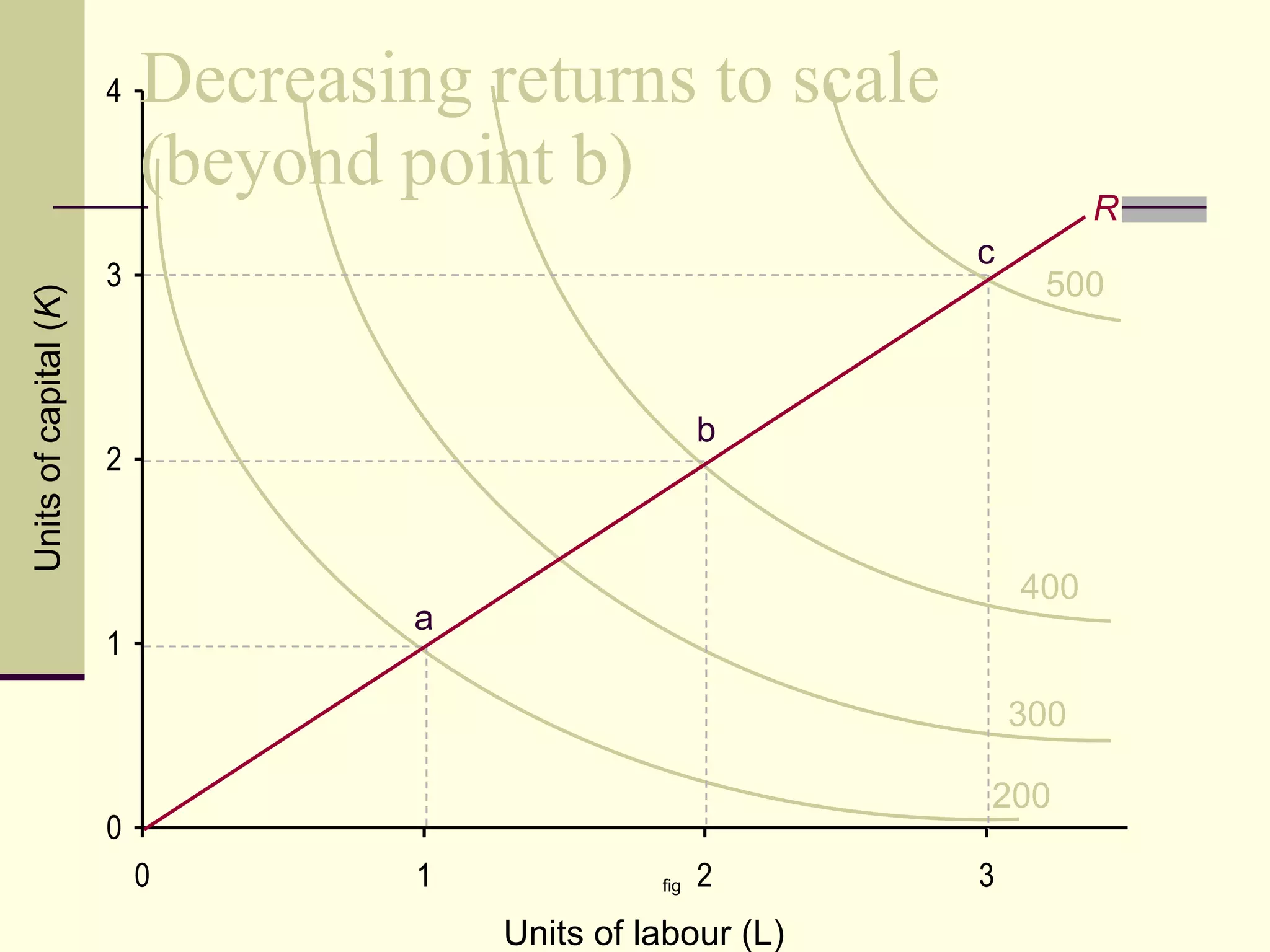
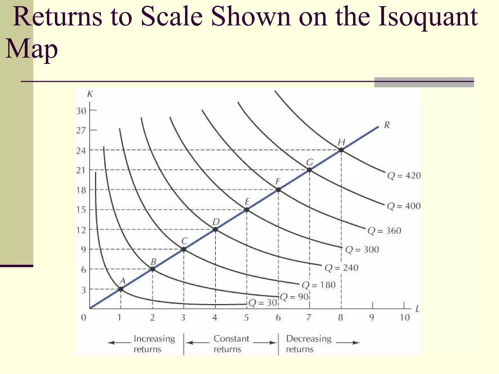
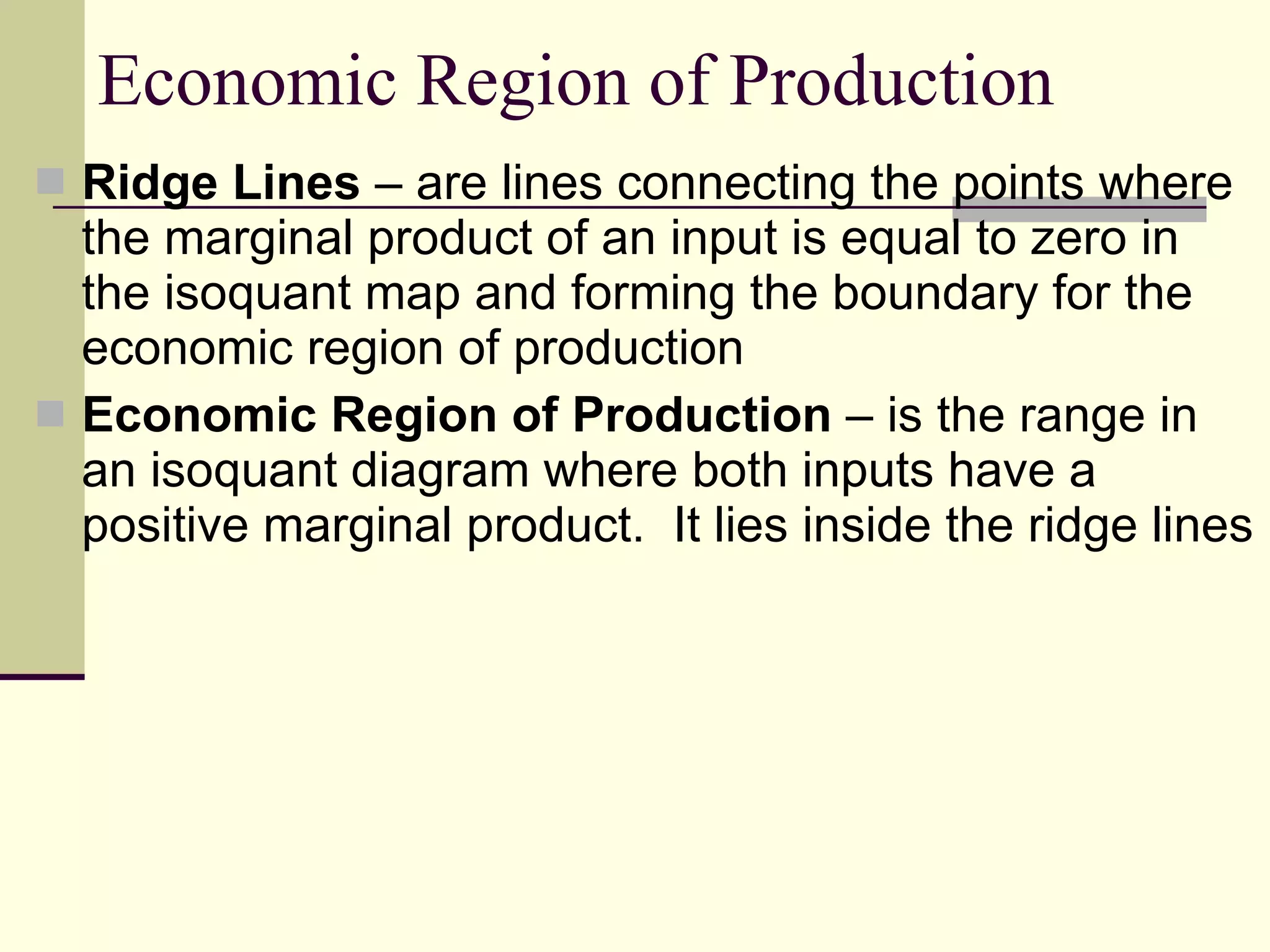
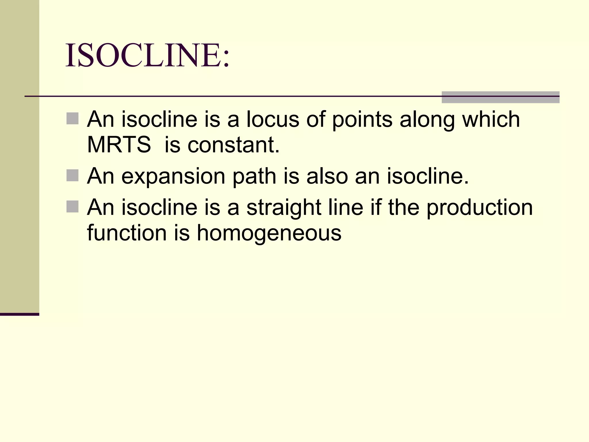
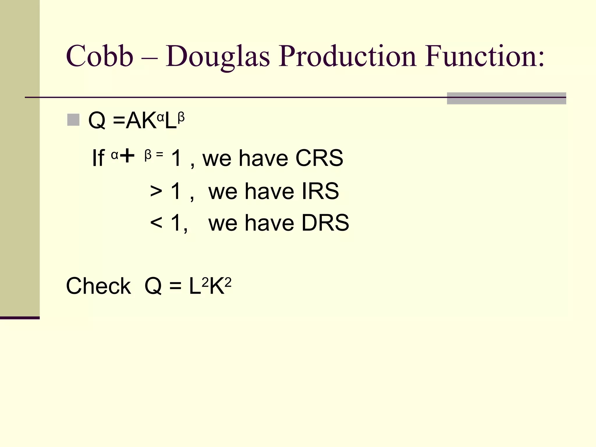
The document discusses production theory, which forms the foundation of supply theory. It covers key concepts such as: 1) Short-run vs long-run production and the fixed and variable nature of inputs. 2) Production functions and the relationship between total, average, and marginal product. 3) The law of diminishing marginal returns and the three stages of production. 4) Isoquants, isocost lines, and how firms determine optimal input combinations to minimize costs.

1. THEORY OF PRODUCTION

2. Production theory forms the foundation for the theory of supply Managerial decision making involves four types of production decisions: 1. Whether to produce or to shut down 2. How much output to produce 3. What input combination to use 4. What type of technology to use

3. Production involves transformation of inputs such as capital, equipment, labor, and land into output - goods and services Production theory can be divided into short run theory or long run theory.

4. Long run and short run: The Long Run is distinguished from the short run by being a period of time long enough for all inputs, or factors of production, to be variable as far as an individual firm is concerned The Short Run , on the other hand, is a period so brief that the amount of at least one input is fixed The length of time necessary for all inputs to be variable may differ according to the nature of the industry and the structure of a firm

5. Production Function A production function is a table or a mathematical equation showing the maximum amount of output that can be produced from any specified set of inputs, given the existing technology. The total product curve for different technology is given below. x Q Q = output x = inputs

6. Production Function continued Q = f(X 1 , X 2 , …, X k ) where Q = output X 1 , …, X k = inputs For our current analysis, let’s reduce the inputs to two, capital (K) and labor (L): Q = f(L, K)

7. DEFINITIONS: In the short run, capital is held constant. Average product is total product divided by the number of units of the input Marginal product is the addition to total product attributable to one unit of variable input to the production process fixed input remaining unchanged. MP = TP N – TP N-1

8. Short run labour Total product Average product Marginal product 1 10 10 10 2 24 12 14 3 39 13 15 4 52 13 13 5 61 12.2 9 6 66 11 5 7 66 9.4 0 8 64 8 -2

9. Marginal and Average product: Marginal product at any point is the slope of the total product curve Average product is the slope of the line joining the point on the total product curve to the origin. When Average product is maximum, the slope of the line joining the point to the origin is also tangent to it.

10. P: Maximum Average Product Q & R : Same Average Product

11. Both AP and MP first rise, reach a maximum and then fall. MP = AP when AP is maximum. MP may be negative if Variable input is used too intensively. Law of diminishing marginal productivity states that in the short run if one input is fixed, the marginal product of the variable input eventually starts falling

12. Law of Diminishing Returns (Diminishing Marginal Product) Holding all factors constant except one , the law of diminishing returns says that: As additional units of a variable input are combined with a fixed input, at some point the additional output (i.e., marginal product) starts to diminish e.g. trying to increase labor input without also increasing capital will bring diminishing returns

13. Three stages of production: Stage 1: Till average product becomes maximum Stage 2: till MP =zero Stage 3: MP is negative

14. Three Stages of Production in Short Run AP,MP X Stage I Stage II Stage III AP X MP X

15. Long run production: Section 2:

16. Production in the Long-Run All inputs are now considered to be variable (both L and K in our case) How to determine the optimal combination of inputs? To illustrate this case we will use production isoquants . An isoquant is a curve showing all possible combinations of inputs physically capable of producing a given fixed level of output.

17. An isoquant fig Units of K 40 20 10 6 4 Units of L 5 12 20 30 50 Point on diagram a b c d e a Units of labour ( L ) Units of capital ( K ) b c d

18. Isoquants and the Production Function Isoquant is a curve that shows the various combinations of two inputs that will produce a given level of output Slope of an isoquant indicates the rate at which factors K and L can be substituted for each other while a constant level of production is maintained. The slope is called Marginal Rate of Technical Substitution (MRTS)

19. Properties of Isoquants There is a different isoquant for every output rate the firm could possibly produce with isoquants farther from the origin indicating higher rates of output Along a given isoquant, the quantity of labor employed is inversely related to the quantity of capital employed  isoquants have negative slopes

20. Properties of Isoquants Isoquants do not intersect. Since each isoquant refers to a specific rate of output, an intersection would indicate that the same combination of resources could, with equal efficiency, produce two different amounts of output Isoquants are usually convex to the origin  any isoquant gets flatter as we move down along the curve

21. Substitutability of Inputs Three general types of shapes that an isoquant might have are: The isoquants are right angles, indicating that inputs a and b must be used in fixed proportions and therefore are not substitutable e.g Yeast and flour for a specific type of bread

22. Substitutability of Inputs Perfect Substitutes – in this case input a can be substituted for input b at a fixed rate as indicated by the straight line isoquants (which have a constant slope and MRS) Ie. Honey and brown sugar are often nearly perfect substitutes, Natural gas and fuel oil are close substitutes in energy production

23. Isoquant Maps for Perfect Substitutes and Perfect Complements

24. Substitutability of Inputs Imperfect Substitutes – and the rate at which input b can be given up in return for one more unit of input a while maintaining the same level of output (the MRS) diminished as the amount of input a being used increases Ie. In farming, harvestors and labour for harvesting grain provide an example of a diminishing MRS, and in general capital and labour are imperfect substitutes.

25. The Marginal Rate of Technical Substitution

26. Marginal Rate of Technical Substitution The absolute value of the slope of the isoquant is the marginal rate of technical substitution, MRTS, between two resources Thus, the MRTS is the rate at which labor substitutes for capital without affecting output  when much capital and little labor are used, the marginal productivity of labor is relatively great and the marginal productivity of capital relatively small  one unit of labor will substitute for a relatively large amount of capital

27. Law of Diminishing Marginal Rate of Technical Substitution :

28. Marginal Rate of Technical Substitution If labor and capital were perfect substitutes in production, the rate at which labor substituted for capital would remain fixed along the isoquant  the isoquant would be a downward sloping straight line Summary Isoquants farther from the origin represent higher rates of output Isoquants slope downward Isoquants never intersect Isoquants are bowed toward the origin

29. Marginal Rate of Technical Substitution Anywhere along the isoquant, the marginal rate of technical substitution of labor for capital equals the marginal product of labor divided by the marginal product of capital, which also equals the absolute value of the slope of the isoquant MRTS = MP L / MP C

30. Isocost Lines Isocost lines show different combinations of inputs which give the same cost At the point where the isocost line meets the vertical axis, the quantity of capital that can be purchased equals the total cost divided by the monthly cost of a unit of capital  TC / r Where the isocost line meets the horizontal axis, the quantity of labor that can be purchased equals the total cost divided by the monthly cost of a unit of labor  TC / w The slope of the isocost line is given by Slope of isocost line = -(TC/r)/(TC/w) = -w/r

31. Choice of Input Combinations The profit maximizing firm wants to produce its chosen output at the minimum cost  it tries to find the isocost closest to the origin that still touches the chosen isoquant. Isocost Line - is a line that shows the various combinations of two inputs that can be bought for a given dollar cost. The equation for an isocost line is: C =L. P L +K. P K

32. Maximizing Output for a given cost

33. Minimizing Cost subject to given Output

34. Expansion Path If we imagine a set of isoquants representing each possible rate of output, and given the relative cost of resources, we can then draw isocost lines to determine the optimal combination of resources for producing each rate of output

35. Expansion Path leads to Total Cost Curve An expansion path is a long-run concept (because all inputs can change) Each point on the expansion path represents a cost-minimizing combination of inputs Given input prices, each point represents a total cost of producing a given level of output when the entrepreneur can choose any input combination he or she want

36. Expansion Path If the relative prices of resources change, the least-cost resource combination will also change  the firm’s expansion path will change For example, if the price of labor increases, capital becomes relatively less expensive  the efficient production of any given rate of output will therefore call for less labor and more capital

37. Returns to Scale Is large scale production more efficient than small scale production for a certain market?  Is a market better served by many small firms or a few large ones? The returns to scale concept describes the relationship between scale and efficiency.

38. Returns to Scale The returns to scale concept is an inherently long run concept. Increasing returns to scale : a production function for which any given proportional change in all inputs leads to a more than proportional change in output.

39. Returns to Scale Constant returns to scale : a production function for which a proportional change in all inputs causes output to change by the same proportion. Decreasing returns to scale : a production function for which a proportional change in all inputs causes a less than proportional change in output.

40. The Distinction between Diminishing Returns and Decreasing Returns to Scale Diminishing returns to scale is a short run concept that refers to the case in which one input varies while all others are held fixed. Decreasing returns to scale is a long run concept that refers to the case in which all inputs are varied by the same proportion.

41. Constant returns to scale fig Units of capital ( K ) Units of labour (L) 200 300 400 500 600 R a b c

42. Increasing returns to scale (beyond point b) fig Units of capital ( K ) Units of labour (L) 200 300 400 500 600 a b c R 700

43. Decreasing returns to scale (beyond point b) fig Units of capital ( K ) Units of labour (L) 200 300 400 500 a b c R

44. Returns to Scale Shown on the Isoquant Map

45. Economic Region of Production There are certain combinations of inputs that the firm should not use in the long run no matter how cheap they are (unless the firm is being paid to use them) These input combinations are represented by the portion of an isoquant curve that has a positive slope

46. Economic Region of Production A positive sloped isoquant means that merely to maintain the same level of production, the firm must use more of both inputs if it increases its use of one of the inputs The marginal product of one input is negative, and using more of that input would actually cause output to fall unless more of the other input were also employed.

47. Economic Region of Production Ridge Lines – are lines connecting the points where the marginal product of an input is equal to zero in the isoquant map and forming the boundary for the economic region of production Economic Region of Production – is the range in an isoquant diagram where both inputs have a positive marginal product. It lies inside the ridge lines

48. Homogeneous Production function: If both factors of production are increased by proportion λ , and if new level of output Q* can be expressed as a function of λ to any power v, and the initial output , i.e. Q* = λ V Q then the function is homogeneous and v is the degree of homogeneity. For example , check the function Q = 4L+3K 2

49. If the production function is homogeneous , the expansion path is a straight line. Check the homogeneity of the following functions: Q = 4L +3K Q= 4KL Q =4KL+K

50. A simple production function is the Cobb-Douglas form Three parameters: A ,  , and  The Cobb-Douglas production function has CRS if  +  =1 The Cobb-Douglas production function has increasing (decreasing) returns to scale if  +  If  =  =½, we have the square root production function

51. ISOCLINE: An isocline is a locus of points along which MRTS is constant. An expansion path is also an isocline. An isocline is a straight line if the production function is homogeneous

52. Cobb – Douglas Production Function: Q =AK α L β If α + β = 1 , we have CRS > 1 , we have IRS < 1, we have DRS Check Q = L 2 K 2