Production Function

1. 7/21/2022 Raksha Singh
Cobb-Douglas Production
Function
Raksha Singh
Professor
Department of Economics
Central University
IGNTU

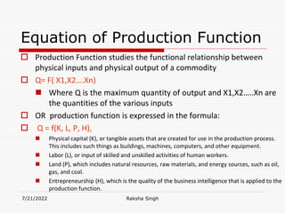
2. Production and Cost Function
UNIT III
7/21/2022 Raksha Singh
Production and Cost
function: law of variable
proportions. Returns to
scale production,
properties of linear
homogeneous
production function,
cobb douglas and ces
derivation of cost
function

3. Equation of Production Function
 Production Function studies the functional relationship between
physical inputs and physical output of a commodity
 Q= F( X1,X2….Xn)
 Where Q is the maximum quantity of output and X1,X2…..Xn are
the quantities of the various inputs
 OR production function is expressed in the formula:
 Q = f(K, L, P, H),
 Physical capital (K), or tangible assets that are created for use in the production process.
This includes such things as buildings, machines, computers, and other equipment.
 Labor (L), or input of skilled and unskilled activities of human workers.
 Land (P), which includes natural resources, raw materials, and energy sources, such as oil,
gas, and coal.
 Entrepreneurship (H), which is the quality of the business intelligence that is applied to the
production function.
7/21/2022 Raksha Singh

4. Equation of Production
Function
 Where the quantity produced is a function of the combined
input amounts of each factor. Of course, not all businesses
require the same factors of production or number of inputs.
 Another form of the production function reduces the inputs to
just labor and physical capital.
 If there are only two inputs, labor L and capital k, Equation will
be
 Q= F(L,K).
 The formula for this form in which labor and capital are the
two factors of production with the greatest impact on the
quantity of output.
7/21/2022 Raksha Singh

5. Cobb Douglas production function
 The Cobb-Douglas production function is based on the
empirical study of the American manufacturing industry
made by Paul H. Douglas and C.W. Cobb.
 It studies the relation between the input and the output.
 It is a linear homogeneous production function of degree
one which takes into account two inputs, labour and
capital, for the entire output of the .manufacturing
industry.
7/21/2022 Raksha Singh

6. Cobb-Douglas production function…
 Mathematician Charles Cobb and the economist Paul
Douglas who used it to consider the relative importance of
the two input factors, labour and capital, in manufacturing
output in the USA over the period 1899 to 1922.
 The cobb douglas production function is that type of
production function wherein an input can be substituted
by others to a limited extent.
 In their original model, Cobb and Douglas restrict the
output-elasticity parameters α1 and α2 to the range
αi∈(0,1) and to sum to one, which implies constant returns
to scale. The function is thus
7/21/2022 Raksha Singh

7. Algebraic Expression

7/21/2022 Raksha Singh

8. The Cobb-Douglas production
function :basic formula

7/21/2022 Raksha Singh

9. Question

7/21/2022 Raksha Singh

10. Answer
 Assume A = 40, a = 0.3 and b= 0.7 , K = 3 and L = 5
 Therefore,
 Q = 40 (3)0.3 (5)0.7 ( By applying log both the sides)
log Q = log 40 + 0.3 log 3 + 0.7 log 5
log Q = 1.6020 + (0.3 X 0.4771) + (0.7 X 0.6989)
log Q = 1.6020 + 0.1431 + 0.4892
log Q = 2.2343
 Now, we will take the antilog of the above to get the value of Q.
antilog log Q = antilog 2.2343
 Q = 171.5141
7/21/2022 Raksha Singh

11. CD applied as UTILITY function
 The Cobb-Douglas functional form is not only used in the
theory of production but it has also become standard in
microeconomic consumer theory where it is applied as a
utility function,
 where Y becomes U for utility. The xi then represent items
of consumption and, when the utility function is maximised
subject to a budget constraint, the values for αi indicate
how the individual will optimally distribute budget among
items.
7/21/2022 Raksha Singh

12. Properties of Cobb Douglas Production
Function

7/21/2022 Raksha Singh

13. Properties of Cobb Douglas
Production Function…
 It makes use of parameters a and b, which signifies the
elasticity coefficients of output for inputs, labour and
capital, respectively.
 Output elasticity coefficient is the change in output that
occurs due to adjustment in capital while keeping labour at
constant.
 It acts as a homogeneous production function, whose
degree can be calculated by the value obtained after adding
values of a and b.
 If the resultant value of a+b is 1, it implies that the degree of
homogeneity is 1 and indicates the constant returns to scale.
7/21/2022 Raksha Singh

14. Explanation with graph

7/21/2022 Raksha Singh

15. Explanation with graph….
7/21/2022 Raksha Singh
 The C-D production function showing
constant returns to scale is depicted in Figure
20.
 Labour input is taken on the horizontal axis
and capital on the vertical axis.
 To produce 100 units of output, ОС, units of
capital and OL units of labour are used. If the
output were to be doubled to 200, the inputs
of labour and capital would have to be
doubled. ОС is exactly double of ОС1 and of
OL2 is double o f OL2.

16. Explanation with graph….
 Similarly, if the output is to be raised three-
fold to 300, the units of labour and capital will
have to be increased three-fold. OC3 and OL3
are three times larger than ОС1, and OL1,
respectively. Another method is to take the
scale line or expansion path connecting the
equilibrium points Q, P and R. OS is the scale
line or expansion path joining these points.
 It shows that the isoquants 100, 200 and 300
are equidistant. Thus, on the OS scale line OQ
= QP = PR which shows that when capital and
labour are increased in equal proportions, the
output also increases in the same proportion.
7/21/2022 Raksha Singh

17. Criticisms of C-D Production
Function:
 The C-D production function has been criticised by Arrow,
Chenery, Minhas and Solow as discussed below:
 1. The C-D production function considers only two inputs, labour
and capital, and neglects some important inputs, like raw
materials, which are used in production. It is, therefore, not
possible to generalize this function to more than two inputs.
 2. In the C-D production function, the problem of measurement
of capital arises because it takes only the quantity of capital
available for production. But the full use of the available capital
can be made only in periods of full employment. This is
unrealistic because no economy is always fully employed.
7/21/2022 Raksha Singh

18. Criticisms of C-D Production
Function….
 3. The C-D production function is criticised because it shows
constant returns to scale. But constant returns to scale are not an
actuality, for either increasing or decreasing returns to scale are
applicable to production.
 4. It is not possible to change all inputs to bring a proportionate
change in the outputs of all the industries. Some inputs are scarce
and cannot be increased in the same proportion as abundant
inputs. On the other hand, inputs like machines, entrepreneurship,
etc. are indivisible. As output increases due to the use of indivisible
factors to their maximum capacity, per unit cost falls.
7/21/2022 Raksha Singh

19. Log tables
7/21/2022 Raksha Singh

20. 7/21/2022 Raksha Singh

21. 7/21/2022 Raksha Singh

22. References
 Ahuja, H. L. (2018). Advanced Economic Theory. New Delhi: S Chand .
 Dewett, K. K. (2001). Modern Economic Theory. New Delhi: S Chand & Company Ltd.
 Jhingan, M. (2017). Advanced Economic Theory-. Delhi: vrinda publications (P) Ltd.
 https://www.toppr.com/guides/fundamentals-of-economics-and-
management/theory-of-production/law-of-variable-proportions/
7/21/2022 Raksha Singh
 Ahuja, H. L. (2018). Advanced Economic Theory. New Delhi: S Chand .
 Dewett, K. K. (2001). Modern Economic Theory. New Delhi: S Chand & Company Ltd.
 Jhingan, M. (2017). Advanced Economic Theory-. Delhi: vrinda publications (P) Ltd.
 https://www.toppr.com/guides/fundamentals-of-economics-and-
management/theory-of-production/law-of-variable-proportions/

23. Thank You
7/21/2022 Raksha Singh
 https://www.youtube.com/watch?v=gXv8KN3JtJs&list=TLPQMDMx
MjIwMjDWwvSTEx1ksg&index=4
 https://www.youtube.com/watch?v=2cibM0oywiU
 https://www.youtube.com/watch?v=4yEmcXkJ8Tk