
Recommended
More Related Content
Similar to 22424roduction Slides 33623-1.ppt
Similar to 22424roduction Slides 33623-1.ppt (20)
More from MuskanKhan320706
More from MuskanKhan320706 (19)
Recently uploaded
Recently uploaded (20)
22424roduction Slides 33623-1.ppt
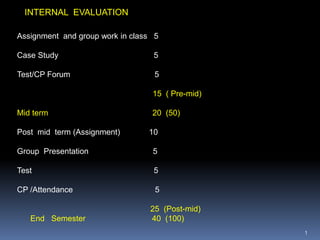
- 1. 1 INTERNAL EVALUATION Assignment and group work in class 5 Case Study 5 Test/CP Forum 5 15 ( Pre-mid) Mid term 20 (50) Post mid term (Assignment) 10 Group Presentation 5 Test 5 CP /Attendance 5 25 (Post-mid) End Semester 40 (100)
- 2. 2
- 3. 3 Production involves transformation of inputs such as capital, equipment, labor, and land into output - goods and services In this production process, the manager is concerned with efficiency in the use of the inputs - technical vs. economical efficiency PRODUCTION -CONCEPT 1
- 4. Two Concepts of Efficiency Economic efficiency: occurs when the cost of producing a given output is as low as possible Technological efficiency: occurs when it is not possible to increase output without increasing inputs 4
- 5. Concept 2-Production Function A production function is purely technical relation which connects factor inputs & outputs. It describes the transformation of factor inputs into outputs at any particular time period. 5 Q = f( L,K,R,Ld,T,t) where Q = output R= Raw Material L= Labour Ld = Land K= Capital T = Technology t = time For our current analysis, let’s reduce the inputs to two, capital (K) and labor (L): Q = f(L, K)
- 6. Short-Run and Long-Run Production concept 3 LAW OF VARIABLE PROPORTIONS In the short run some inputs are fixed and some variable e.g. the firm may be able to vary the amount of labor, but cannot change the amount of capital in the short run we can talk about factor productivity law of variable proportion/law of diminishing returns 6
- 7. 7 In the long run all inputs become variable e.g. the long run is the period in which a firm can adjust all inputs to changed conditions in the long run we can talk about returns to scale and isoquants Concept -4 ISOQUANTS-LONG RUN
- 8. Short-Run Changes in Production Factor Productivity 8 Units of K Employed Output Quantity (Q) 8 37 60 83 96 107 117 127 128 7 42 64 78 90 101 110 119 120 6 37 52 64 73 82 90 97 104 5 31 47 58 67 75 82 89 95 4 24 39 52 60 67 73 79 85 3 17 29 41 52 58 64 69 73 2 8 18 29 39 47 52 56 52 1 4 8 14 20 27 24 21 17 1 2 3 4 5 6 7 8 Units of L Employed How much does the quantity of Q change, when the quantity of L is increased?
- 9. Relationship Between Total, Average, and Marginal Product: Short-Run Analysis Labor variable-concept 5 Total Product (TP) = total quantity of output Average Product (AP) = total product per total input Marginal Product (MP) = change in quantity when one additional unit of input used 9
- 10. The Marginal Product of Labor- concept 6 The marginal product of labor is the increase in output obtained by adding 1 unit of labor but holding constant the inputs of all other factors Marginal Product of L: MPL= Q/L (holding K constant) Average Product of L: APL= Q/L (holding K constant) 10
- 11. Law of Diminishing Returns (Diminishing Marginal Product) CONCEPT-7 11 The law of diminishing returns states that when more and more units of a variable input are applied to a given quantity of fixed inputs, the total output may initially increase at an increasing rate and then at a constant rate but it will eventually increases at diminishing rates. Assumptions. The law of diminishing returns is based on the following assumptions: (i) the state of technology is given (ii) labour is homogenous and (iii) input prices are given.
- 12. Total and Marginal Product 12 30 90 130 161 184 196 Total Product Q from hiring fourth worker Q from hiring third worker Q from hiring second worker Q from hiring first worker increasing marginal returns diminishing marginal returns Units of Output Number of Workers 6 2 3 4 5 1
- 13. 13 CASE ON HEALTHCARE PRODUCTION FUNCTION- LAW OF DIMINISHING RETURNS
- 14. 14 CONCEPT-PRODUCTION CONCEPT 2- LAW OF VARIABLE PROPORTIONS (SHORT RUN AND PRODUCTION FUNCTION)- (CASE ON CALL CENTRE) BEHAVIOUR OF TP, MP and AP with dig and example CONCEPT 3- LAW OF DIMINISHING RETURNS(-CASE ON HEALTHCARE) CONCEPT 4-LONG RUN PRODUCTION FUNCTION- ISOQUANT (CASE ON ENERGY INPUT) CONCEPT 5-ISO COST LINE – Equation SHIFTS AND ROTATION OF ISOCOST LINE CONCEPT 6- PRODUCER EQUILIBRIUM CONCEPT 7-RETURNS TO SCALE – INCREASING, CONSTANT, DIMINISHING –(CASE ON CARPET INDUSTRY IN US) COBB DOUGLOUS PRODUCTION FUNCTION
- 15. 15 CONCEPT -8-TYPES OF COST- CASELET CONCEPT 9 – SHORT RUN COST CURVES CONCEPT -LONG RUN COST CURVES CONCEPT 7-RETURNS TO SCALE – INCREASING, CONSTANT, DIMINISHING –(CASE ON CARPET INDUSTRY IN US) COBB DOUGLOUS PRODUCTION FUNCTION,SIMPLE NUMERICALS COSTS ARE A MIRROR IMAGE OF PRODUCTION
- 16. 16 Case - CALL CENTRE- LAW OF VARIABLE PROPORTIONS HEALTHCARE PRODUCTION FUNNCTION –LAW OF DIMINISHING RETURNS
- 17. 17 Three Stages of Production Stages Labor Total Average Marginal of Unit Product Product Product Production (X) (Q or TP) (AP) (MP) 1 24 24 24 2 72 36 48 I 3 138 46 66 Increasing 4 216 54 78 Returns 5 300 60 84 6 384 64 84 7 462 66 78 8 528 66 66 II 9 576 64 48 Diminishing 10 600 60 24 Returns 11 594 54 -6 III 12 552 46 -42 Negative Returns
- 18. 18 1, 24 2, 72 3, 138 4, 216 5, 300 6, 384 7, 462 8, 528 9, 576 10, 600 11, 594 12, 552 1, 24 2, 36 3, 46 4, 54 5, 60 6, 64 7, 66 8, 66 9, 64 10, 60 11, 54 12, 46 1, 24 2, 48 3, 66 4, 78 5, 84 6, 84 7, 78 8, 66 9, 48 10, 24 11, -6 12, -42 0 2 4 6 8 10 12 14 SHORT RUN PRODUCTION FUNCTION Total Product Average Product Marginal Product CAPITAL(K) is constant and LABOUR (L) is variable
- 19. Three Stages of Production in Short Run (Earlier slide also) 19 AP,MP X Stage I Stage II Stage III APX MPX •TPL Increases at increasing rate. •MP Increases at decreasing rate. •AP is increasing and reaches its maximum at the end of stage I •TPL Increases at Diminshing rate. •MPL Begins to decline. •TP reaches maximum level at the end of stage II, MP = 0. •APL declines • TPL begins to decline •MP becomes negative •AP continues to decline CONCEPT -8
- 20. Short-Run Analysis of Total, Average, and Marginal Product If MP > AP then AP is rising If MP < AP then AP is falling MP = AP when AP is maximized TP maximized when MP = 0 20
- 21. 21 CASE ON CALL CENTRE- LAW OF VARIABLE PROPORTIONS 3 STAGES OF PRODUCTION
- 22. Application of Law of Diminishing Returns: It helps in identifying the rational and irrational stages of operations. It gives answers to question – How much to produce? What number of workers to apply to a given fixed inputs so that the output is maximum? Stage 2- call centre 22
- 23. 23 Today’s class
- 24. 24 Theory of Consumer Behaviour Theory of Production LDMU LDMR Indifference curve Isoquant Two commodities X &Y Two factors L&K Properties Same for both Slope of IC MRS xy Slope of Isoquant:MRTS LK Budget line is constraint Slope= Px/Py Isocost line is constraint Slope= w/r Consumer Equilibrium Producer equilibrium Tangency of budget line with IC curve Tangency of Isocost line with Isoquant AIM: CONSTRAINED OPTIMISATION Maximise consumer satisfaction Maximise production subject to cost Subject to budget constraint
- 25. Production in the Long-Run concept 9 All inputs are now considered to be variable (both L and K in our case) How to determine the optimal combination of inputs? To illustrate this case we will use production isoquants. An isoquant is a locus of all technically efficient methods or all possible combinations of inputs for producing a given level of output. 25
- 26. Production Table 26 Units of K Employed Output Quantity (Q) 8 37 60 83 96 107 117 127 128 7 42 64 78 90 101 110 119 120 6 37 52 64 73 82 90 97 104 5 31 47 58 67 75 82 89 95 4 24 39 52 60 67 73 79 85 3 17 29 41 52 58 64 69 73 2 8 18 29 39 47 52 56 52 1 4 8 14 20 27 24 21 17 1 2 3 4 5 6 7 8 Units of K Employed of L Isoquant Units of K Employed
- 27. Isoquant -Illustration 27 0 1 2 3 4 5 6 7 0 1 2 3 4 5 6 Capital lABOUR ISOQUANT ISOQUA L K MRTS 2 6 3 4 2 4 3 1 5 2.5 0.5
- 28. Properties of Isoquants- Concept 10 Isoquants have a negative slope. Isoquants are convex to the origin. Isoquants cannot intersect or be tangent to each other. Upper Isoquants represents higher level of output 28
- 29. The degree of imperfection in substitutability is measured with marginal rate of technical substitution (MRTS- Slope of Isoquant): MRTS = L/K (in this MRTS some of L is removed from the production and substituted by K to maintain the same level of output) 29 Marginal Rate of Technical Substitution MRTS (Concept 11)
- 30. Isoquant Map (Concept 12) Isoquant map is a set of isoquants presented on a two dimensional plain. Each isoquant shows various combinations of two inputs that can be used to produce a given level of output. Figure : Isoquant Map Labour X Capital Y Y O X IQ4 IQ3 IQ2 IQ1 30
- 31. We will use isoquant map (1) and isocost line (2) (Concept 13) Figure : Isoquant Map (1) Capital Y K O L 3x 2x x1 Figure : Isoquant Line (2) K O L C/W C/r B A 31 The cost line is defined by cost equation C= (r) (k) + (w) (L) W wage rate r= price of capital serviceIIiiI
- 32. : the firm attempts either to minimize the cost of producing a given level of output or to maximize the output attainable with a given level of cost. Both optimization problems lead to same rule for the allocation of inputs and choice of technology 32 CONCEPT -CONSTRAINED OPTIMISATION PROBLEM (Concept 14)
- 33. Case I Maximization of output subject to cost constraint Labour 0 L1 K1 C x3 x2 X1 A B Capital 33
- 34. Case II Minimization of cost for given level of output 34 e K 0 L1 K1 L X
- 35. Condition for Equilibrium (concept 15) At point of tendency slope of isocost line (w/r ) = slope of isoquant. (MPL/MPK) The isoquants should be convex to origin 35
- 36. K 3X 2X X L 0 EXPANSION PATH Locus of (Producers equilibrium) Tangency points of Isocost and Isoquants E1 E2 E3 (Concept 16)
- 37. 37 LONG RUN PRODUCTION FUNCTION (Caselet on Energy) Energy and other inputs substitution using Isoquants and Isocost lines Energy becomes costlier what would happen to the isocost line and isoquant
- 38. 38 C C0 5 5 7 10 a b Rate of other inputs Rate Of Energy input CASELET 10 : 7 5:5
- 39. Laws of Returns to Scale CONCEPT 17 It explains the behavior of output in response to a proportional and simultaneous change in input. When a firm increases both the inputs, there are three technical possibilities – (i) TP may increase more than proportionately – Increasing RTS (ii) TP may increase proportionately – constant RTS (iii) TP may increase less than proportionately – diminishing RTS 39
- 41. 41 LDMR exists- TP increases at an increasing rate then diminishing rate and reaches maximium and then falls MP declines and reaches 0 and then becomes negative AP declines continuously Simple Numericals(Calculate MP and AP and show whether Dimishing returns occur Numbers of workers Number of chairs(Q) MP ( Q/L) AP (Q/L) 1 10 2 18 3 24 4 28 5 30 6 30 7 28 8 25
- 42. 42 If w= 3 and r= 2 and cost constraint equals 30 draw the Isocost line. If a)w decreases to 2 indicate the rotation b) If cost constraint expand to 60 indicate the shift C= rk +wl 30 = 2k + 3L 60= 2K+3L
- 43. 43 Returns to scale (Next class) Caslet on carpet Industry Cobb Douglas Production function Types of Cost Cost concepts Relationship between production and cost Short run cost curves Long run cost curves