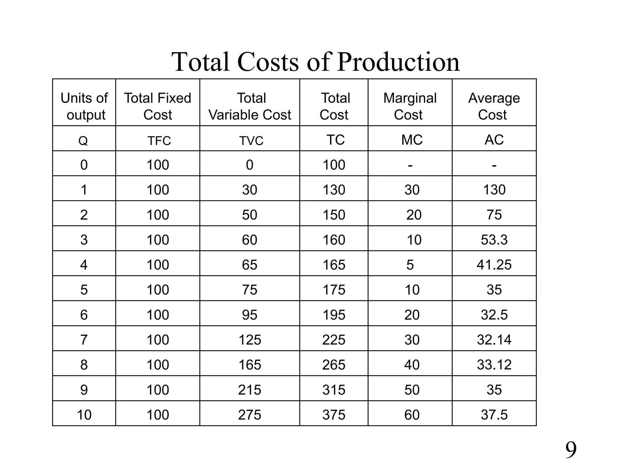
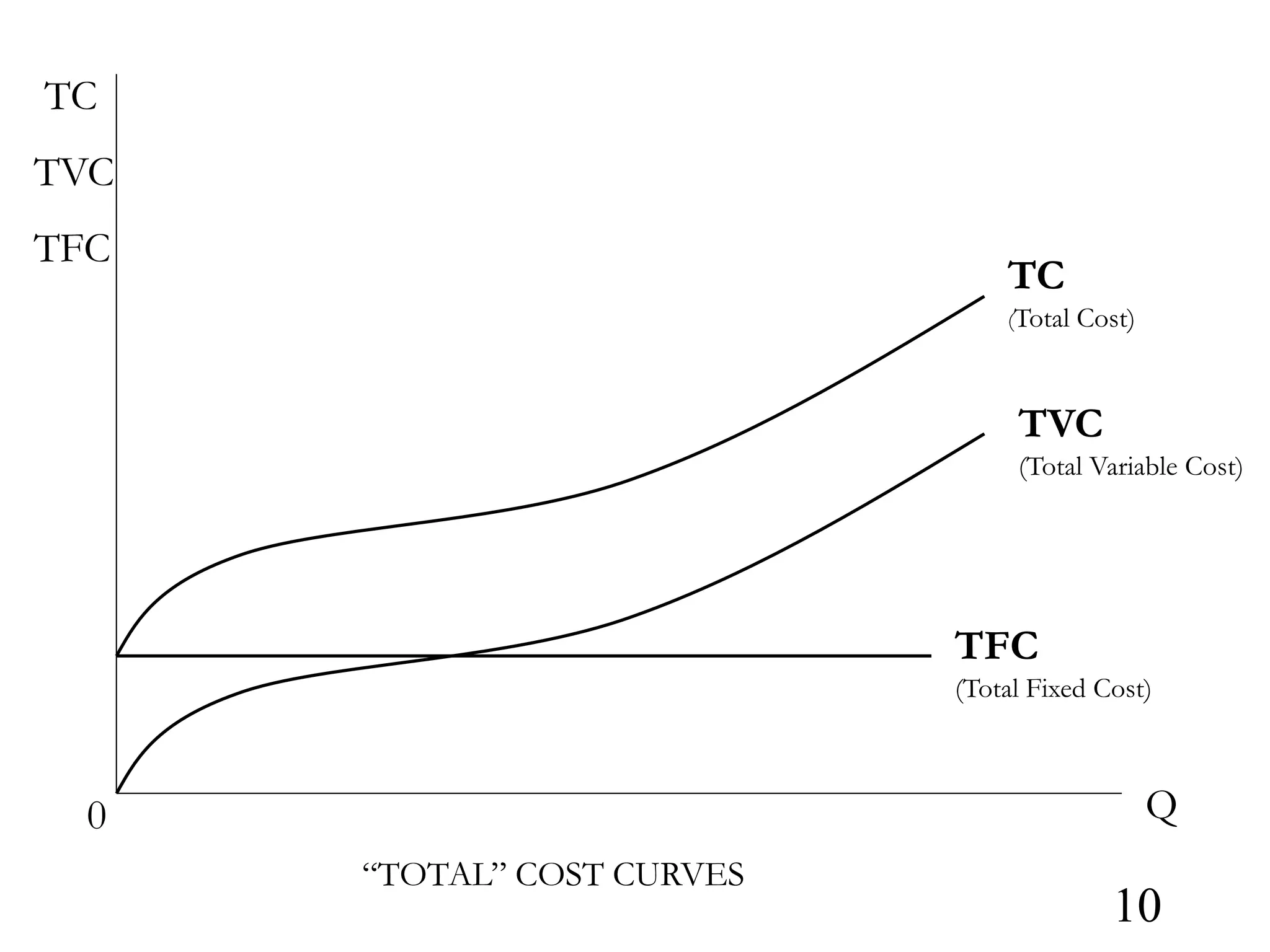
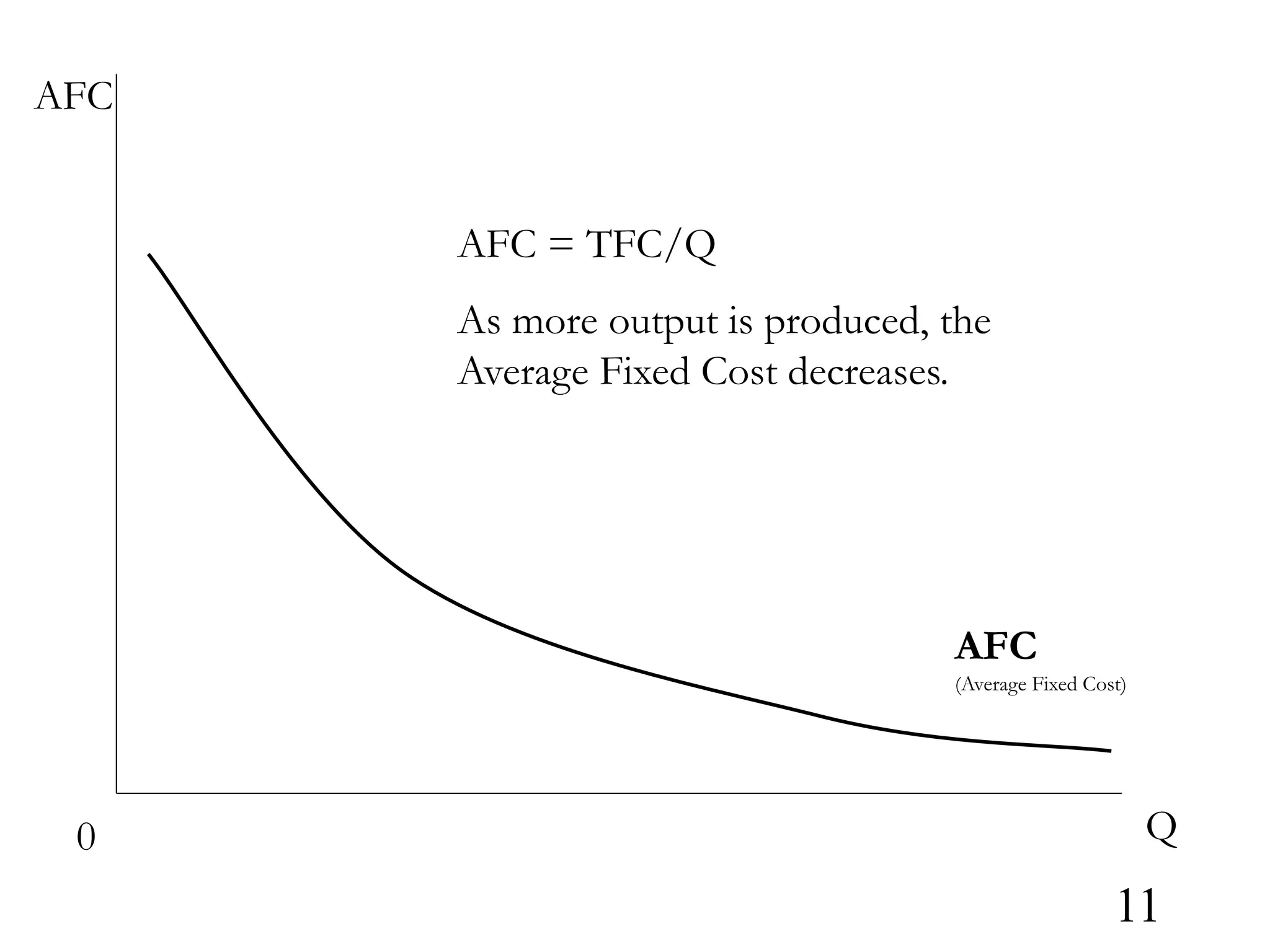
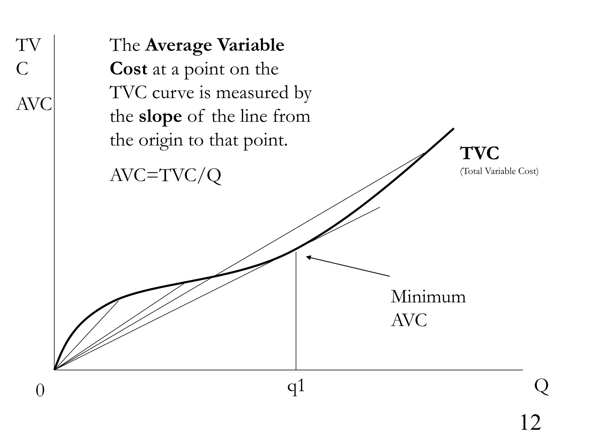
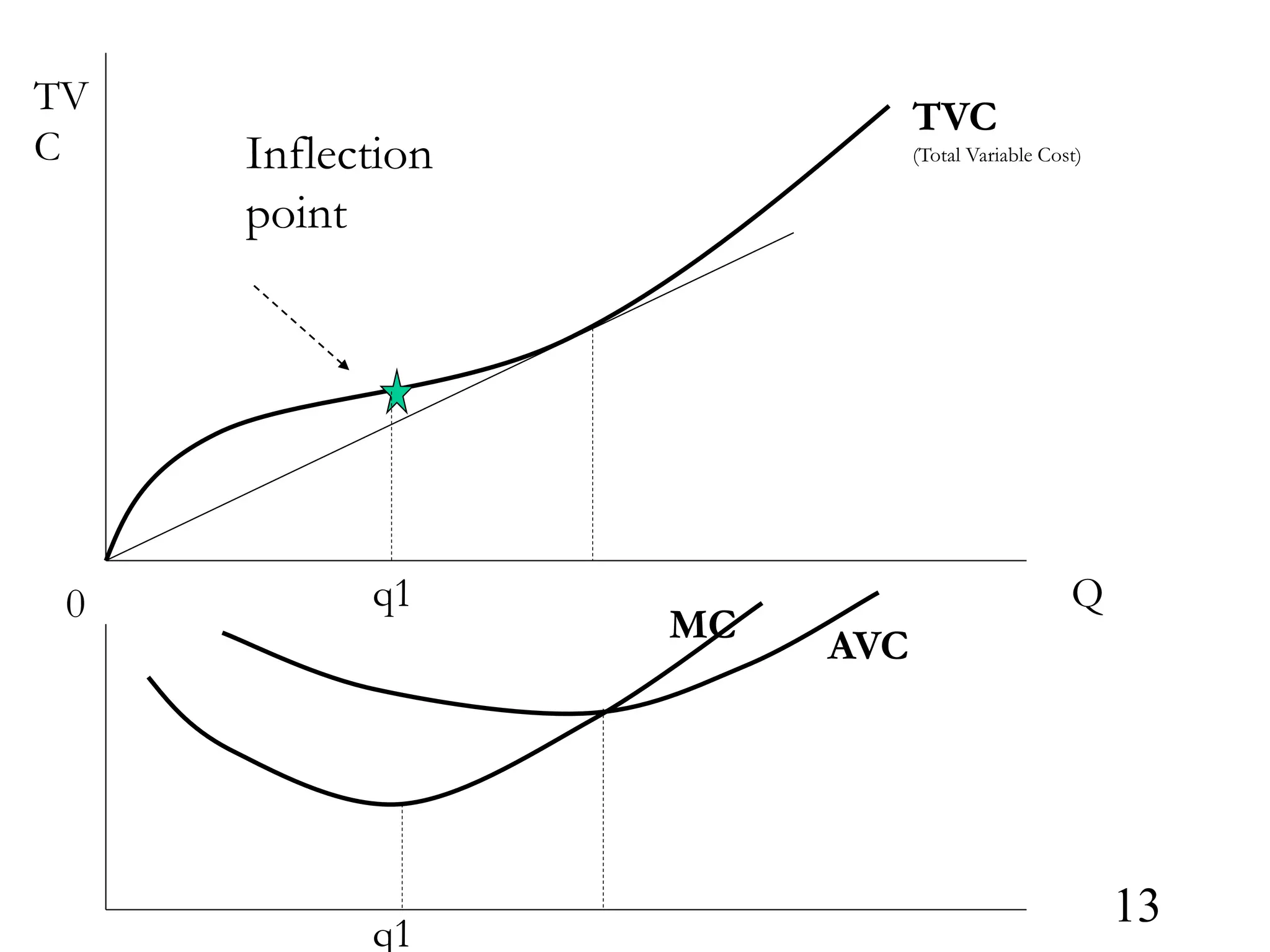
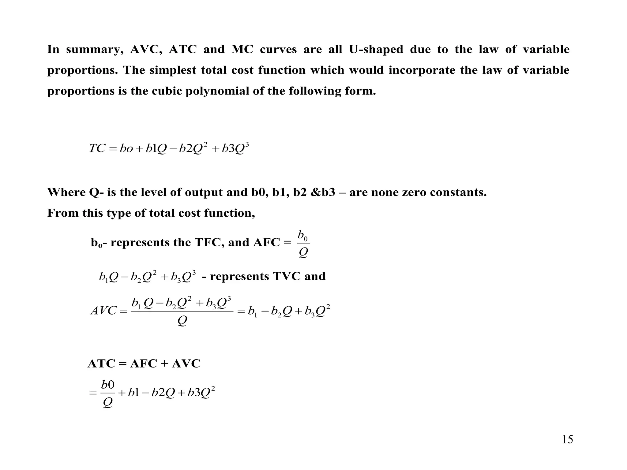
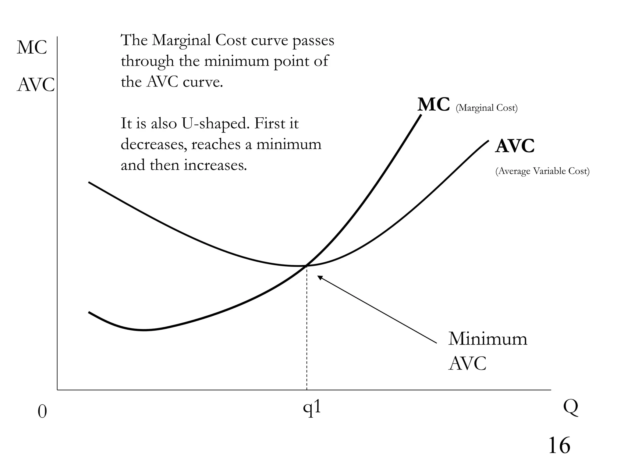
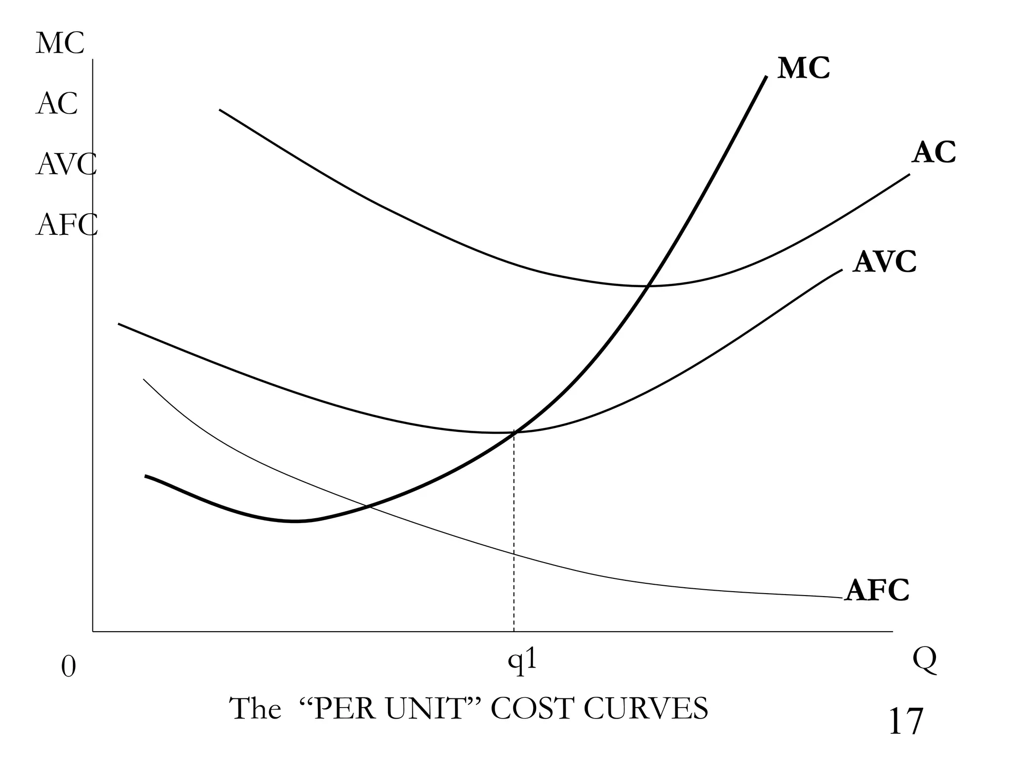
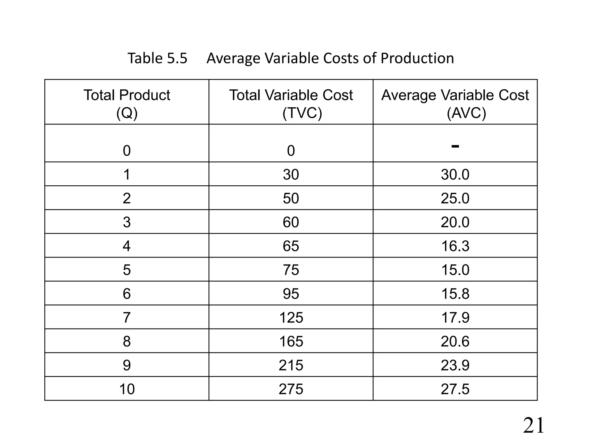
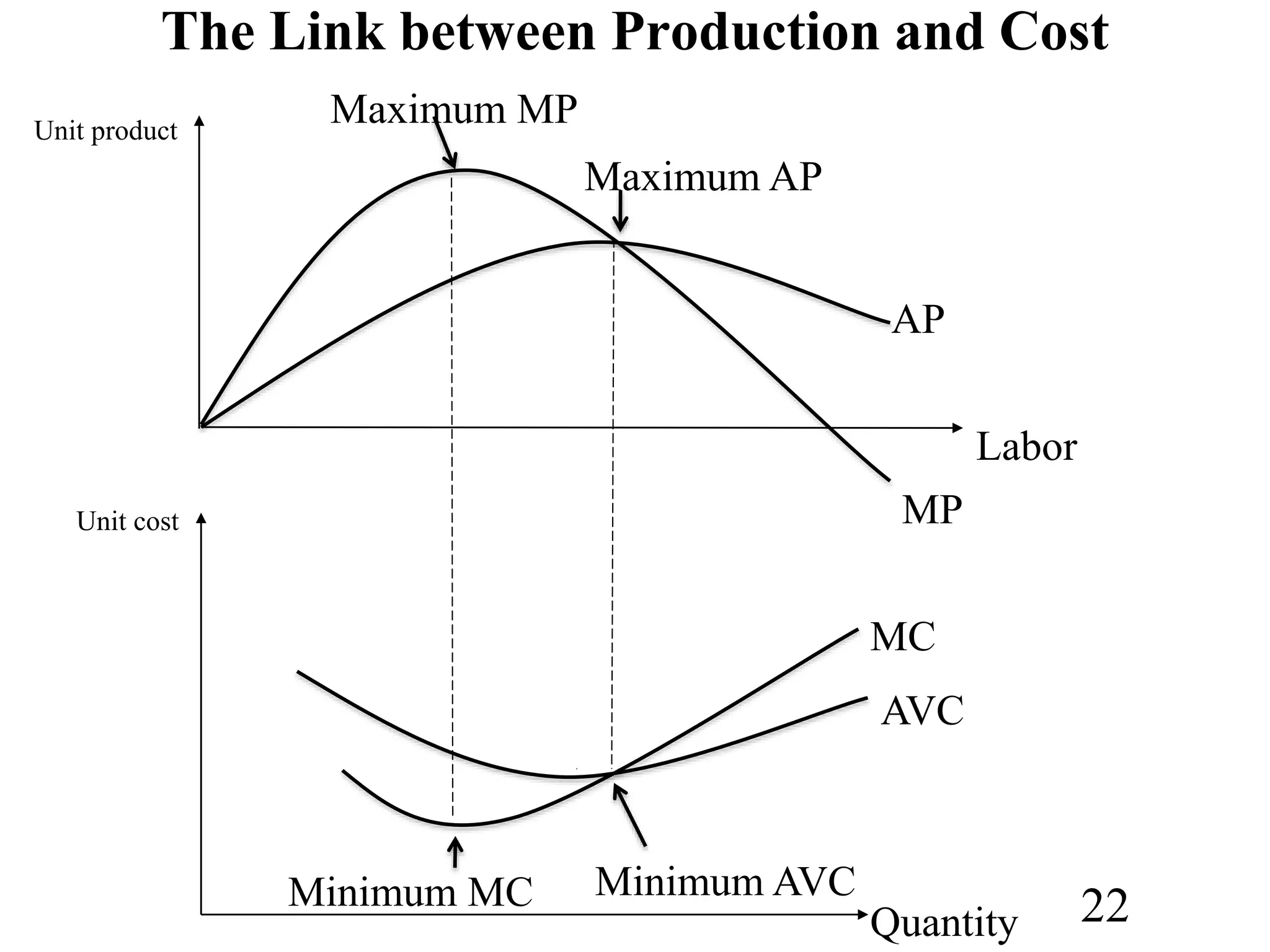
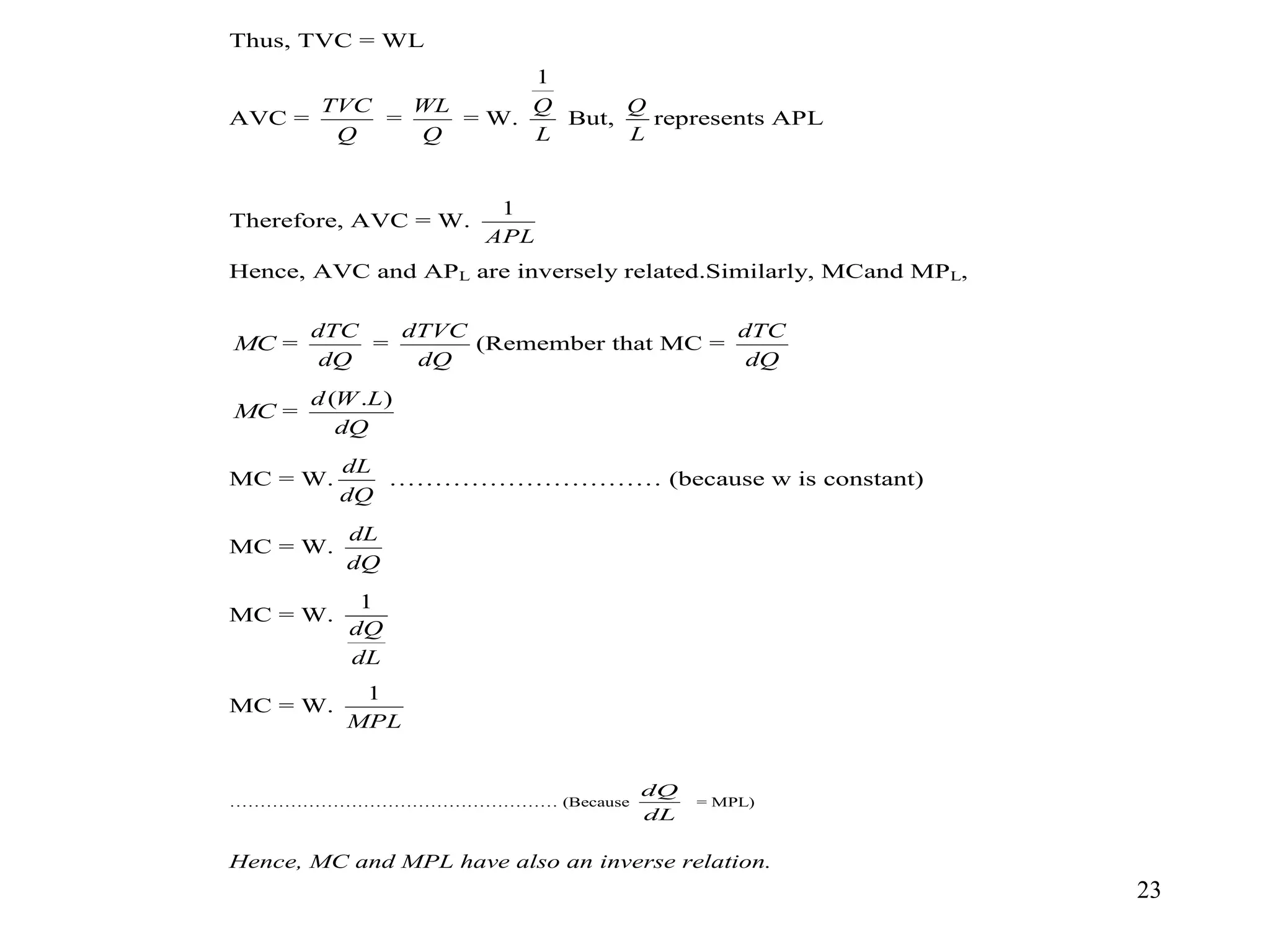
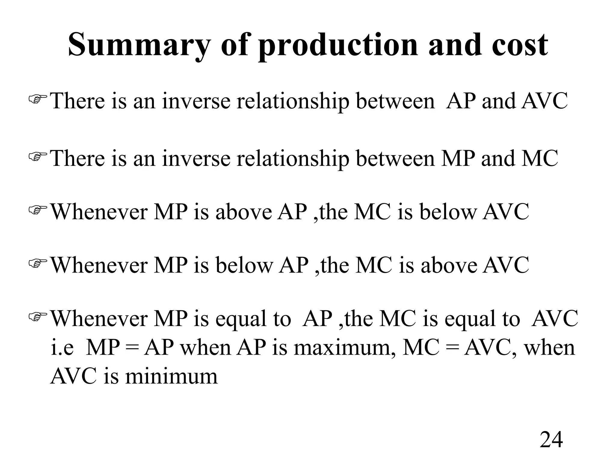
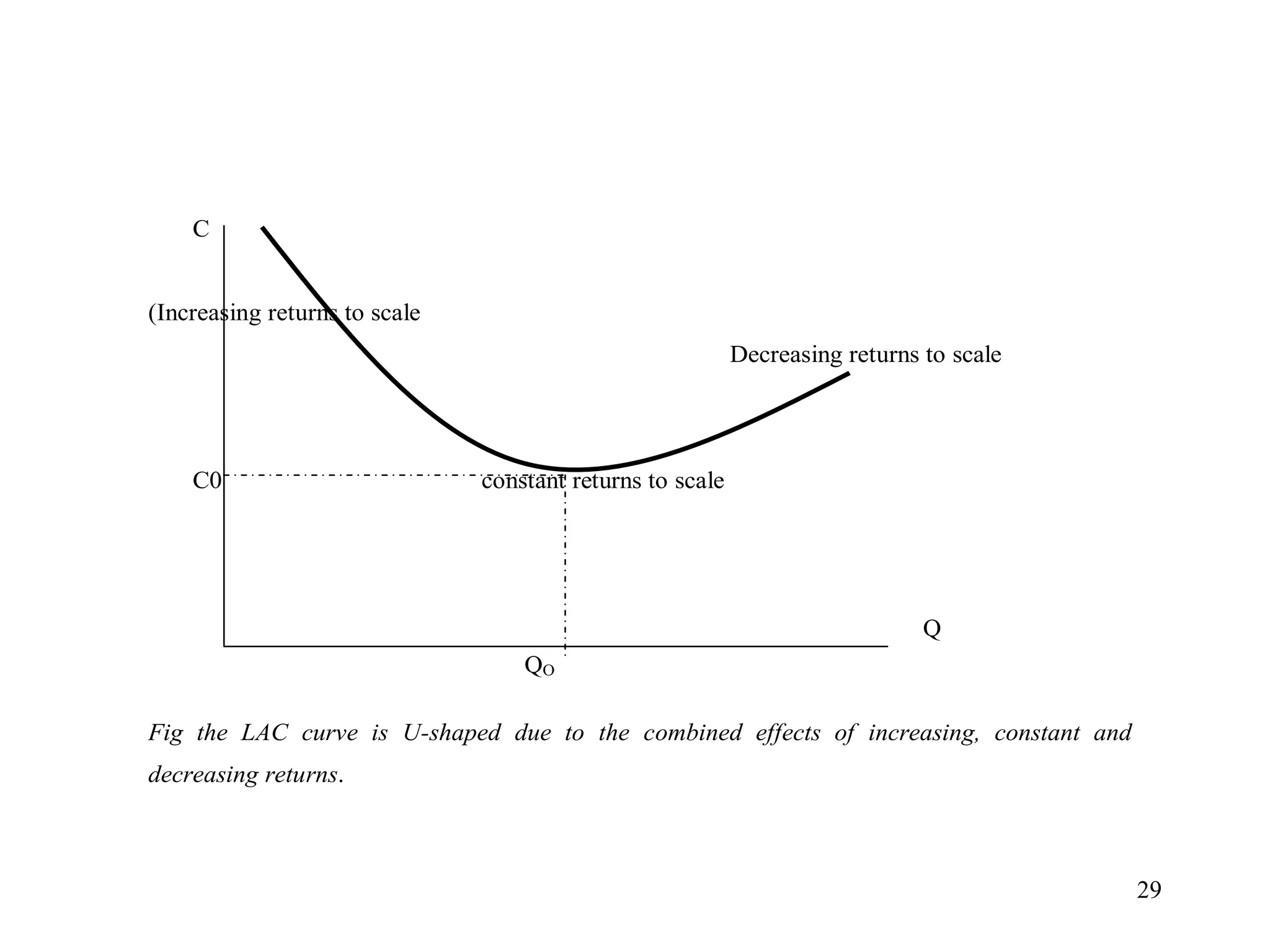
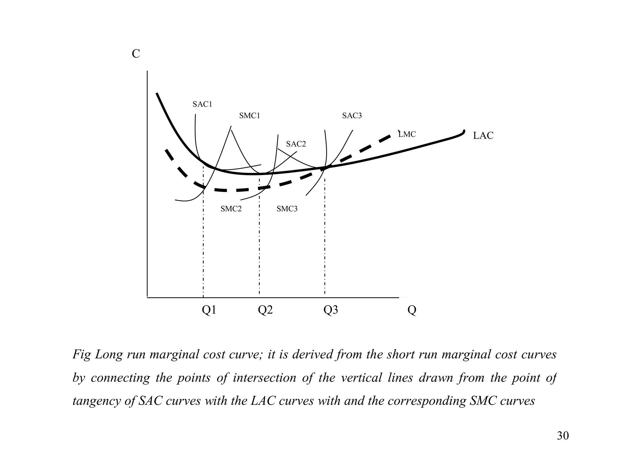
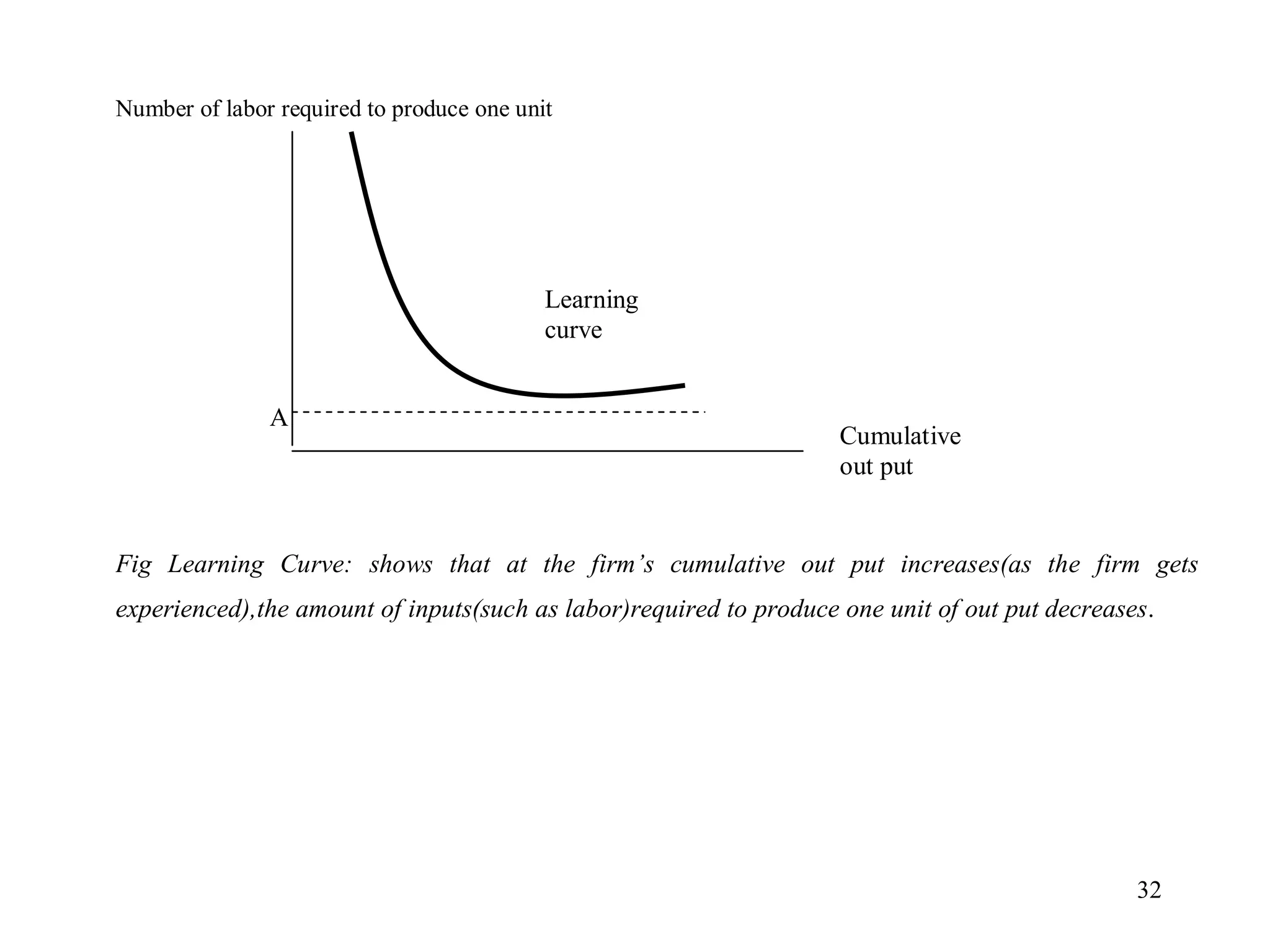
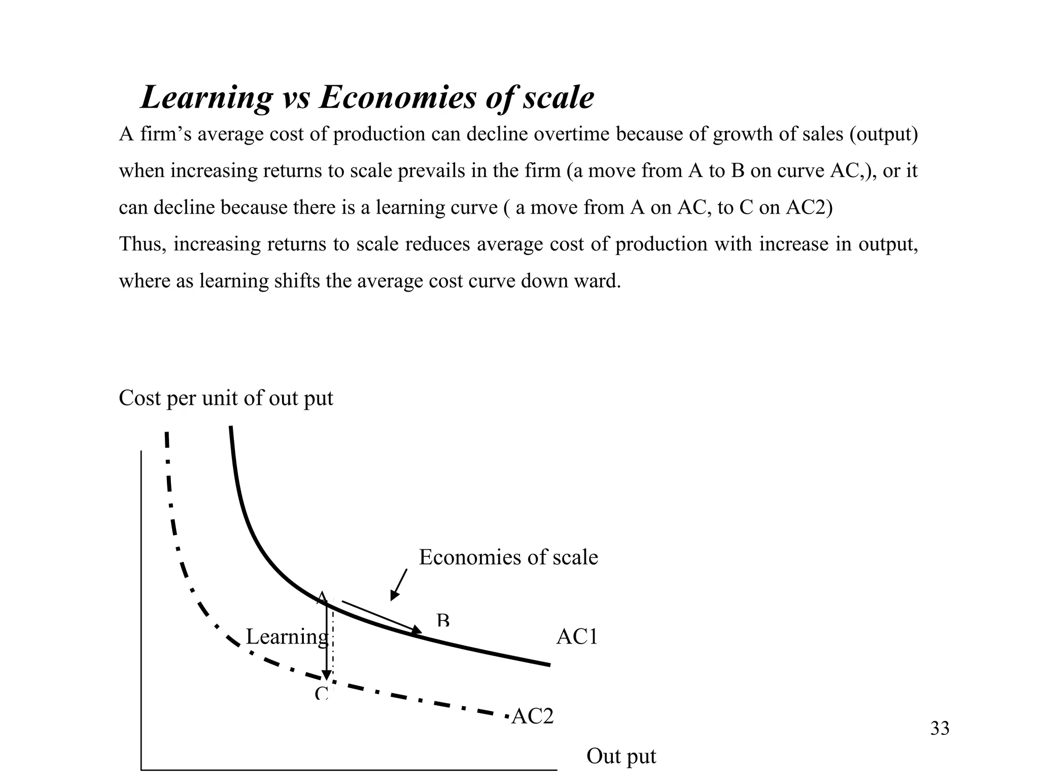
Theory of Costs
• Cost : is the monetary value of inputs used in the
production of an item.
Two types of cost of a product
• Social cost: is the cost of producing an item to the
society
• Private cost: is the cost of producing an item to the
individual producer.
1
Private cost of production can be measured
in two ways
 Economic cost & accounting cost
A. Economic cost: the cost of all inputs used
to produce the item.
• Economic cost = Explicit costs + Implicit
cost
– Explicit costs – costs paid in cash
– Implicit cost – imputed cost of self-owned or self
employed resources based on their opportunity costs.
2
Implicit Vs Explicit Costs
– Opportunity cost principle - the economic cost of
an input used in a production process is the value of
output sacrificed elsewhere
The opportunity cost of an input is the value of
forgone income in best alternative employment
B. Accounting cost: refers to the cost of purchased
inputs only
It is the explicit cost of production only
3
Cost Concepts (Short-run cost of production)
1. Total Fixed Cost (TFC)
2. Total Variable Cost (TVC)
3. Total Cost (TC = TVC+TFC)
4. Average Fixed Cost (AFC = TFC/Q)
5. Average Variable Cost (AVC = TVC/Q)
6. Average Total Cost (AC = AFC+AVC)
7. Marginal Cost (MC= ∆TVC/∆Q
4
Cost concept …
• Total fixed cost (TFC) or fixed cost (FC) refers
to those costs that do not vary as the firm changes
its output level
– Examples: the payment or rent for land, buildings and
machinery, Depreciation, Interest, Taxes (property),
Insurance
– The fixed cost is independent of the level of output
produced.
– Graphically, it is depicted as a horizontal line
5
• Total variable cost (TVC) or Variable cost
(VC) refers to the cost that changes as the
amount of output produced is changed
– Examples - purchases of raw materials, payments
to workers, electricity bills, fuel and power costs
– Total variable cost increases as the amount of
output increases
• If no output is produced, then total variable cost is
zero; the larger the output, the greater the total
variable cost
6
• Total cost (TC) is the sum of total fixed cost and total
variable cost, i.e., TC = TFC + TVC
• As the level of output increases, total cost of the firm
also increases.
• Marginal cost (MC) is the additional cost incurred
from producing an additional unit of output:
MC = TC/Q
or MC = TVC/Q
7
Selected attributes
• MC is generally increasing.
• MC crosses ATC and AVC at their
minimum point.
• If MC is below the average cost, Average
cost will be decreasing.
• If MC is above the average cost, Average
cost will be increasing.
8
Total Costs of Production
Units of
output
Total Fixed
Cost
Total
Variable Cost
Total
Cost
Marginal
Cost
Average
Cost
Q TFC TVC TC MC AC
0 100 0 100 - -
1 100 30 130 30 130
2 100 50 150 20 75
3 100 60 160 10 53.3
4 100 65 165 5 41.25
5 100 75 175 10 35
6 100 95 195 20 32.5
7 100 125 225 30 32.14
8 100 165 265 40 33.12
9 100 215 315 50 35
10 100 275 375 60 37.5
9
Q
0
TFC
(Total Fixed Cost)
TC
TVC
TFC
TVC
(Total Variable Cost)
TC
(Total Cost)
“TOTAL” COST CURVES
10
Q
0
AFC
(Average Fixed Cost)
AFC
AFC = TFC/Q
As more output is produced, the
Average Fixed Cost decreases.
11
Q
0
TV
C
AVC
TVC
(Total Variable Cost)
q1
The Average Variable
Cost at a point on the
TVC curve is measured by
the slope of the line from
the origin to that point.
AVC=TVC/Q
Minimum
AVC
12
Q
0
TV
C
MC
q1
Inflection
point
TVC
(Total Variable Cost)
q1
AVC
13
Q
0
AVC
AVC
(Average Variable Cost)
q1
The Average Variable Cost
is U shaped. First it
decreases, reaches a
minimum and then
increases.
Minimum
AVC
14
15
In summary, AVC, ATC and MC curves are all U-shaped due to the law of variable
proportions. The simplest total cost function which would incorporate the law of variable
proportions is the cubic polynomial of the following form.
3
2
3
2
1 Q
b
Q
b
Q
b
bo
TC 



Where Q- is the level of output and b0, b1, b2 &b3 – are none zero constants.
From this type of total cost function,
bo- represents the TFC, and AFC =
Q
b0
3
3
2
2
1 Q
b
Q
b
Q
b 
 - represents TVC and
2
3
2
1
3
3
2
2
1
Q
b
Q
b
b
Q
Q
b
Q
b
Q
b
AVC 





ATC = AFC + AVC
2
3
2
1
0
Q
b
Q
b
b
Q
b




Q
0
MC
AVC
AVC
(Average Variable Cost)
q1
The Marginal Cost curve passes
through the minimum point of
the AVC curve.
It is also U-shaped. First it
decreases, reaches a minimum
and then increases.
Minimum
AVC
MC (Marginal Cost)
16
Q
0
MC
AC
AVC
AFC
AVC
q1
MC
AFC
AC
The “PER UNIT” COST CURVES 17
18
Finally, the MC curve passes through the minimum point of both ATC and AVC curves.
This can be shown by using calculus.
Suppose the TC = f (Q)
Slope of
But f (Q) is MC and Q1 (or dQ/dQ) =1
)
(
))
(
(
Q
f
dQ
Q
f
d
MC 

Q
Q
f
Q
TC
AC
)
(


2
)
(
.
))
(
(
(Q))
(f
d
Q
Q
f
Q
Q
Q
f
dQ
d
AC



Q
Q
Q
f
Q
MC
Q
AC
)
(
2
f(Q)
-
MC.Q



19
Thus, slope of
Slope AC =   AC
Q
Q
f
where
AC
MC
Q


)
(
,
1
Now,
i) when MC<AC, the slope of AC is negative, i.e. AC curve is decreasing (initial
stage of production)
ii) When MC >AC, the slope of AC is positive, i.e. the AC curve is increasing
(after optimal combination of fixed and variable inputs.
iii) When MC = AC, the slope of AC is zero, i.e. the AC curve is at its minimum
point.
The relationship between AVC and MC can be shown in a similar fashion.
Table 5.4 Average Cost of Production
(Q) (TC) (AC)
0 100 -
1 130 130.00
2 150 75.00
3 160 53.33
4 165 41.25
5 175 35.00
6 195 32.50
7 225 32.14
8 265 33.13
9 315 35.00
10 375 37.50
20
Total Product
(Q)
Total Variable Cost
(TVC)
Average Variable Cost
(AVC)
0 0 -
1 30 30.0
2 50 25.0
3 60 20.0
4 65 16.3
5 75 15.0
6 95 15.8
7 125 17.9
8 165 20.6
9 215 23.9
10 275 27.5
Table 5.5 Average Variable Costs of Production
21
The Link between Production and Cost
Maximum MP
Maximum AP
Minimum AVC
Minimum MC
Unit product
Unit cost
AP
MP
MC
AVC
Labor
Quantity 22
23
Thus, TVC = WL
AVC =
Q
TVC
=
Q
WL
= W.
L
Q
1
But,
L
Q
represents APL
Therefore, AVC = W.
APL
1
Hence, AVC and APL are inversely related.Similarly, MCand MPL,
MC =
dQ
dTC
=
dQ
dTVC
(Remember that MC =
dQ
dTC
MC =
dQ
L
W
d )
.
(
MC = W.
dQ
dL
………………………… (because w is constant)
MC = W.
dQ
dL
MC = W.
dL
dQ
1
MC = W.
MPL
1
……………………………………………… (Because
dL
dQ
= MPL)
Hence, MC and MPL have also an inverse relation.
Summary of production and cost
There is an inverse relationship between AP and AVC
There is an inverse relationship between MP and MC
Whenever MP is above AP ,the MC is below AVC
Whenever MP is below AP ,the MC is above AVC
Whenever MP is equal to AP ,the MC is equal to AVC
i.e MP = AP when AP is maximum, MC = AVC, when
AVC is minimum
24
Cost Curves in the Long Run
• In the long run, the amount of all factors of production
can be varied so that there are no fixed costs.
• The time period corresponding to the long run will be
such a condition that the producers can make all the
necessary changes in the size of the plant.
• Fixed cost will be variable in the long run decision of
production
• When we say that fixed costs vary with the size of the
plant, we mean that all costs behave in the same way as
all other components of the variable costs.
25
The Long run average cost curves
• The long- run average cost curve is an ‘envelope’ of
all the short run ATC curves corresponding to all the
different levels of factors of production that are fixed
in the short- run.
• The LRAC curve is given by the point of tangency to
all the short-run curves representing all the alternative
plant sizes that a firm could be able to build in the
long-run.
• To know it more look at the following graph.
26
LA
C
SAC
1
Q
0
COST
SAC
2
LONG-RUN AVERAGE COST CURVE
SAC
3
SAC
4
SAC
5
SAC
6
27
28
Why is the LAC U-shaped?
The LAC curve is U-shaped due to the laws of returns to
scale(i.e increasing & decreasing returns to scale) that is, as
output expands from a very low levels increasing returns to
scale prevails (i.e., output rises proportionally more than
inputs), & so the cost per-unit of output falls
As output continues expand, the forces of decreasing returns
to scale eventually begin to overtake the forces of increasing
returns to scale & the LAC begins to rise
In general, the reason for the U-shaped ness of the LAC curve
are the existence of increasing returns to scale at initial stage
of expansion decreasing returns to scale at a later stage of
expansion.
29
QO
C
(Increasing returns to scale
Decreasing returns to scale
C0 constant returns to scale
Fig the LAC curve is U-shaped due to the combined effects of increasing, constant and
decreasing returns.
Q
30
LMC LAC
SMC2
SAC2
SMC3
Q3
Q2
Q1
C
Fig Long run marginal cost curve; it is derived from the short run marginal cost curves
by connecting the points of intersection of the vertical lines drawn from the point of
tangency of SAC curves with the LAC curves with and the corresponding SMC curves
SMC1
SAC1
SAC3
Q
31
Dynamic changes in costs: the learning curve
Reason why a large firm may have a lower long-run average cost than a
small firm: increasing returns to scale in production it is tempting to
conclude that firms which enjoy lower average cost over time are
growing firms with increasing returns to scale but this need not be true
In long-run, average cost may decline over time because workers and
managers absorb new technological information as they become more
experienced at their job
That is, as workers get experience their efficiency increases which then
reduces the average and marginal costs of producing a unit of product
A firm’s learns’ over time as cumulative output increases. Managers
can use this learning process to help plan production and forecast future
costs.
32
A
Number of labor required to produce one unit
Fig Learning Curve: shows that at the firm’s cumulative out put increases(as the firm gets
experienced),the amount of inputs(such as labor)required to produce one unit of out put decreases.
Learning
curve
Cumulative
out put
33
Learning vs Economies of scale
A firm’s average cost of production can decline overtime because of growth of sales (output)
when increasing returns to scale prevails in the firm (a move from A to B on curve AC,), or it
can decline because there is a learning curve ( a move from A on AC, to C on AC2)
Thus, increasing returns to scale reduces average cost of production with increase in output,
where as learning shifts the average cost curve down ward.
Cost per unit of out put
Economies of scale
Learning AC1
AC2
Out put
A
C
B

Cost function.ppt

  • 1.
    Theory of Costs •Cost : is the monetary value of inputs used in the production of an item. Two types of cost of a product • Social cost: is the cost of producing an item to the society • Private cost: is the cost of producing an item to the individual producer. 1
  • 2.
    Private cost ofproduction can be measured in two ways  Economic cost & accounting cost A. Economic cost: the cost of all inputs used to produce the item. • Economic cost = Explicit costs + Implicit cost – Explicit costs – costs paid in cash – Implicit cost – imputed cost of self-owned or self employed resources based on their opportunity costs. 2
  • 3.
    Implicit Vs ExplicitCosts – Opportunity cost principle - the economic cost of an input used in a production process is the value of output sacrificed elsewhere The opportunity cost of an input is the value of forgone income in best alternative employment B. Accounting cost: refers to the cost of purchased inputs only It is the explicit cost of production only 3
  • 4.
    Cost Concepts (Short-runcost of production) 1. Total Fixed Cost (TFC) 2. Total Variable Cost (TVC) 3. Total Cost (TC = TVC+TFC) 4. Average Fixed Cost (AFC = TFC/Q) 5. Average Variable Cost (AVC = TVC/Q) 6. Average Total Cost (AC = AFC+AVC) 7. Marginal Cost (MC= ∆TVC/∆Q 4
  • 5.
    Cost concept … •Total fixed cost (TFC) or fixed cost (FC) refers to those costs that do not vary as the firm changes its output level – Examples: the payment or rent for land, buildings and machinery, Depreciation, Interest, Taxes (property), Insurance – The fixed cost is independent of the level of output produced. – Graphically, it is depicted as a horizontal line 5
  • 6.
    • Total variablecost (TVC) or Variable cost (VC) refers to the cost that changes as the amount of output produced is changed – Examples - purchases of raw materials, payments to workers, electricity bills, fuel and power costs – Total variable cost increases as the amount of output increases • If no output is produced, then total variable cost is zero; the larger the output, the greater the total variable cost 6
  • 7.
    • Total cost(TC) is the sum of total fixed cost and total variable cost, i.e., TC = TFC + TVC • As the level of output increases, total cost of the firm also increases. • Marginal cost (MC) is the additional cost incurred from producing an additional unit of output: MC = TC/Q or MC = TVC/Q 7
  • 8.
    Selected attributes • MCis generally increasing. • MC crosses ATC and AVC at their minimum point. • If MC is below the average cost, Average cost will be decreasing. • If MC is above the average cost, Average cost will be increasing. 8
  • 9.
    Total Costs ofProduction Units of output Total Fixed Cost Total Variable Cost Total Cost Marginal Cost Average Cost Q TFC TVC TC MC AC 0 100 0 100 - - 1 100 30 130 30 130 2 100 50 150 20 75 3 100 60 160 10 53.3 4 100 65 165 5 41.25 5 100 75 175 10 35 6 100 95 195 20 32.5 7 100 125 225 30 32.14 8 100 165 265 40 33.12 9 100 215 315 50 35 10 100 275 375 60 37.5 9
  • 10.
    Q 0 TFC (Total Fixed Cost) TC TVC TFC TVC (TotalVariable Cost) TC (Total Cost) “TOTAL” COST CURVES 10
  • 11.
    Q 0 AFC (Average Fixed Cost) AFC AFC= TFC/Q As more output is produced, the Average Fixed Cost decreases. 11
  • 12.
    Q 0 TV C AVC TVC (Total Variable Cost) q1 TheAverage Variable Cost at a point on the TVC curve is measured by the slope of the line from the origin to that point. AVC=TVC/Q Minimum AVC 12
  • 13.
  • 14.
    Q 0 AVC AVC (Average Variable Cost) q1 TheAverage Variable Cost is U shaped. First it decreases, reaches a minimum and then increases. Minimum AVC 14
  • 15.
    15 In summary, AVC,ATC and MC curves are all U-shaped due to the law of variable proportions. The simplest total cost function which would incorporate the law of variable proportions is the cubic polynomial of the following form. 3 2 3 2 1 Q b Q b Q b bo TC     Where Q- is the level of output and b0, b1, b2 &b3 – are none zero constants. From this type of total cost function, bo- represents the TFC, and AFC = Q b0 3 3 2 2 1 Q b Q b Q b   - represents TVC and 2 3 2 1 3 3 2 2 1 Q b Q b b Q Q b Q b Q b AVC       ATC = AFC + AVC 2 3 2 1 0 Q b Q b b Q b    
  • 16.
    Q 0 MC AVC AVC (Average Variable Cost) q1 TheMarginal Cost curve passes through the minimum point of the AVC curve. It is also U-shaped. First it decreases, reaches a minimum and then increases. Minimum AVC MC (Marginal Cost) 16
  • 17.
  • 18.
    18 Finally, the MCcurve passes through the minimum point of both ATC and AVC curves. This can be shown by using calculus. Suppose the TC = f (Q) Slope of But f (Q) is MC and Q1 (or dQ/dQ) =1 ) ( )) ( ( Q f dQ Q f d MC   Q Q f Q TC AC ) (   2 ) ( . )) ( ( (Q)) (f d Q Q f Q Q Q f dQ d AC    Q Q Q f Q MC Q AC ) ( 2 f(Q) - MC.Q   
  • 19.
    19 Thus, slope of SlopeAC =   AC Q Q f where AC MC Q   ) ( , 1 Now, i) when MC<AC, the slope of AC is negative, i.e. AC curve is decreasing (initial stage of production) ii) When MC >AC, the slope of AC is positive, i.e. the AC curve is increasing (after optimal combination of fixed and variable inputs. iii) When MC = AC, the slope of AC is zero, i.e. the AC curve is at its minimum point. The relationship between AVC and MC can be shown in a similar fashion.
  • 20.
    Table 5.4 AverageCost of Production (Q) (TC) (AC) 0 100 - 1 130 130.00 2 150 75.00 3 160 53.33 4 165 41.25 5 175 35.00 6 195 32.50 7 225 32.14 8 265 33.13 9 315 35.00 10 375 37.50 20
  • 21.
    Total Product (Q) Total VariableCost (TVC) Average Variable Cost (AVC) 0 0 - 1 30 30.0 2 50 25.0 3 60 20.0 4 65 16.3 5 75 15.0 6 95 15.8 7 125 17.9 8 165 20.6 9 215 23.9 10 275 27.5 Table 5.5 Average Variable Costs of Production 21
  • 22.
    The Link betweenProduction and Cost Maximum MP Maximum AP Minimum AVC Minimum MC Unit product Unit cost AP MP MC AVC Labor Quantity 22
  • 23.
    23 Thus, TVC =WL AVC = Q TVC = Q WL = W. L Q 1 But, L Q represents APL Therefore, AVC = W. APL 1 Hence, AVC and APL are inversely related.Similarly, MCand MPL, MC = dQ dTC = dQ dTVC (Remember that MC = dQ dTC MC = dQ L W d ) . ( MC = W. dQ dL ………………………… (because w is constant) MC = W. dQ dL MC = W. dL dQ 1 MC = W. MPL 1 ……………………………………………… (Because dL dQ = MPL) Hence, MC and MPL have also an inverse relation.
  • 24.
    Summary of productionand cost There is an inverse relationship between AP and AVC There is an inverse relationship between MP and MC Whenever MP is above AP ,the MC is below AVC Whenever MP is below AP ,the MC is above AVC Whenever MP is equal to AP ,the MC is equal to AVC i.e MP = AP when AP is maximum, MC = AVC, when AVC is minimum 24
  • 25.
    Cost Curves inthe Long Run • In the long run, the amount of all factors of production can be varied so that there are no fixed costs. • The time period corresponding to the long run will be such a condition that the producers can make all the necessary changes in the size of the plant. • Fixed cost will be variable in the long run decision of production • When we say that fixed costs vary with the size of the plant, we mean that all costs behave in the same way as all other components of the variable costs. 25
  • 26.
    The Long runaverage cost curves • The long- run average cost curve is an ‘envelope’ of all the short run ATC curves corresponding to all the different levels of factors of production that are fixed in the short- run. • The LRAC curve is given by the point of tangency to all the short-run curves representing all the alternative plant sizes that a firm could be able to build in the long-run. • To know it more look at the following graph. 26
  • 27.
    LA C SAC 1 Q 0 COST SAC 2 LONG-RUN AVERAGE COSTCURVE SAC 3 SAC 4 SAC 5 SAC 6 27
  • 28.
    28 Why is theLAC U-shaped? The LAC curve is U-shaped due to the laws of returns to scale(i.e increasing & decreasing returns to scale) that is, as output expands from a very low levels increasing returns to scale prevails (i.e., output rises proportionally more than inputs), & so the cost per-unit of output falls As output continues expand, the forces of decreasing returns to scale eventually begin to overtake the forces of increasing returns to scale & the LAC begins to rise In general, the reason for the U-shaped ness of the LAC curve are the existence of increasing returns to scale at initial stage of expansion decreasing returns to scale at a later stage of expansion.
  • 29.
    29 QO C (Increasing returns toscale Decreasing returns to scale C0 constant returns to scale Fig the LAC curve is U-shaped due to the combined effects of increasing, constant and decreasing returns. Q
  • 30.
    30 LMC LAC SMC2 SAC2 SMC3 Q3 Q2 Q1 C Fig Longrun marginal cost curve; it is derived from the short run marginal cost curves by connecting the points of intersection of the vertical lines drawn from the point of tangency of SAC curves with the LAC curves with and the corresponding SMC curves SMC1 SAC1 SAC3 Q
  • 31.
    31 Dynamic changes incosts: the learning curve Reason why a large firm may have a lower long-run average cost than a small firm: increasing returns to scale in production it is tempting to conclude that firms which enjoy lower average cost over time are growing firms with increasing returns to scale but this need not be true In long-run, average cost may decline over time because workers and managers absorb new technological information as they become more experienced at their job That is, as workers get experience their efficiency increases which then reduces the average and marginal costs of producing a unit of product A firm’s learns’ over time as cumulative output increases. Managers can use this learning process to help plan production and forecast future costs.
  • 32.
    32 A Number of laborrequired to produce one unit Fig Learning Curve: shows that at the firm’s cumulative out put increases(as the firm gets experienced),the amount of inputs(such as labor)required to produce one unit of out put decreases. Learning curve Cumulative out put
  • 33.
    33 Learning vs Economiesof scale A firm’s average cost of production can decline overtime because of growth of sales (output) when increasing returns to scale prevails in the firm (a move from A to B on curve AC,), or it can decline because there is a learning curve ( a move from A on AC, to C on AC2) Thus, increasing returns to scale reduces average cost of production with increase in output, where as learning shifts the average cost curve down ward. Cost per unit of out put Economies of scale Learning AC1 AC2 Out put A C B