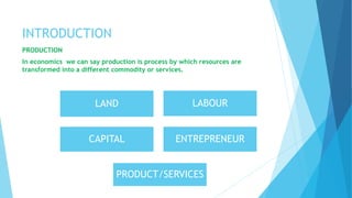
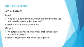
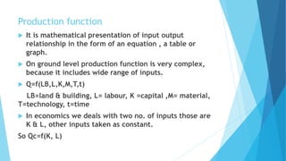
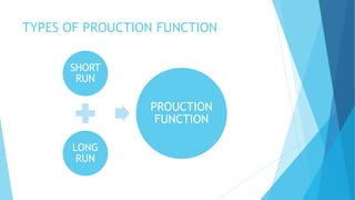
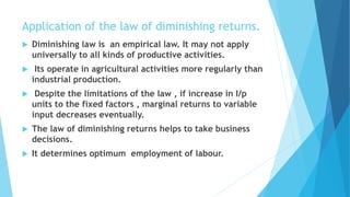
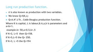
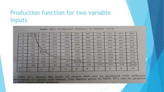
MANAGERIAL ECONOMICS
PRODUCTION & PRODUCTION FUNCTIONS
PRESENTED BY :MUNISH KUMAR
ROLL NO. 16M910
MBA 1ST YEAR
INDEX
 INTRODUCTION
 PRODUCTION FUNCTION WITH ONE VARIABLE
 LAW OF DIMINISHING RETURNS
 OPTIMUM EMPLOYMENT OF LABOUR
 PRODUCTION FUNCTION OF TWO VARIABLE INPUTS
INTRODUCTION
PRODUCTION
In economics we can say production is process by which resources are
transformed into a different commodity or services.
LAND LABOUR
CAPITAL ENTREPRENEUR
PRODUCT/SERVICES
INPUT & OUTPUT
A/C to BAUMOL
Input
 “ Input is simply anything which the firm buys for use
in its production or other process”.
Example: Raw material,labour etc.
Output
 An output is any good or services that comes out of
production process.
Example: Engineer of NIT After 4 year process.
Fixed & variable inputs
Fixed inputs
Fixed inputs whose supply is inelastic in short run, or
input is constant or fixed up to certain level of output.
(e.g. land).
variable inputs
Variable input is one whose supply is elastic in short
run.(labor & raw material, capital).
Production function
 It is mathematical presentation of input output
relationship in the form of an equation , a table or
graph.
 On ground level production function is very complex,
because it includes wide range of inputs.
 Q=f(LB,L,K,M,T,t)
LB=land & building, L= labour, K =capital ,M= material,
T=technology, t=time
 In economics we deals with two no. of inputs those are
K & L, other inputs taken as constant.
So Qc=f(K, L)
TYPES OF PROUCTION FUNCTION
SHORT
RUN
LONG
RUN
PROUCTION
FUNCTION
Short run production function
 It is also term as single input variable function.
 Q is f(K BAR,L) where K bar is constant.
 Q=bl , where b= change in Q/change in L gives
constant return to labour.
 The law of production under these conditions
called “law of variable promotions or law of
return to a variable input.
Law of diminishing returns to a variable
input.
 When more & more variables input are used
with a given quantity of fixed inputs, total o/p
may initially increase at increasing rate, and
then constant rate, but it will eventually
increasing at diminishing rates.
 That’s is the marginal increase in total o/p
decreases eventually when additional units of a
variable factor are used , given quantity of
fixed factors.
Assumption
 Labour is the only variable I/P, K remain constant.
 Labour is homogeneous.
 State of technology is given.
 Input prices are given.
 lets consider Qc=f(L), K constant. For
 Qc=-L³+15L²+10L hypothetical equation for labour o/p
relationship for X Firm. L=5
 So Qc=-125+375+50=300
Cont……
 MARGINAL PRODUCTIVITY OF LABOUR
 MPL=Derivative of Q w.r.t.L=-3L²+30L+10, when we put
L in this equation we get different values of MPL.
 But in this method labour should be perfectly divisible
and delta L approaches to 0.Since L=1 , SO calculas
method is not allowed.
Alternatively ,labour is increased at lest by one. So
MPL=TPL-(TPL-1) where TPL is(Total product).
Average productivity of labour obtained by dividing the
production function by L. that is APL=Qc/L
NO OF
WORKERS
(N)
TOTAL
PRODUCT(TPLIN
MT)
MARGINAL
PRODUCT
(MPL)
AVERAGE
PRODUCT(APL
)
STAGES OF
PRODUCTION
1 24 24 24 INCRESING RETURN
2 72 48 36 DO
3 138 66 46 DO
4 216 78 54 DO
5 300 84 60 DO
6 384 84 64 DO
7 462 78 66 DIMNISHING
8 528 66 66 DO
9 576 48 64 DO
10 600 24 60 DO
11 594 -6 54 NEGATIVE
12 552 -42 46 DO
Application of the law of diminishing returns.
 Diminishing law is an empirical law. It may not apply
universally to all kinds of productive activities.
 Its operate in agricultural activities more regularly than
industrial production.
 Despite the limitations of the law , if increase in I/p
units to the fixed factors , marginal returns to variable
input decreases eventually.
 The law of diminishing returns helps to take business
decisions.
 It determines optimum employment of labour.
Long run production function.
 It is also known as production with two variables.
 We know Q=f(K,L)
 Q=A.Kª.L*b , Cobb-Douglus production function.
Where K is capital, L is labour,& A,a,b is parameters and
a+b=1.
example A= 50,a=0.5,b=.5
If K=2, L=5 then Q=158.
If K=5,L=5 the Q= 250.
If K=3, L =5 the Q=194
Production function for two variable
inputs
PRODUCTION& PRODUCTION FUNCTION

PRODUCTION& PRODUCTION FUNCTION

  • 1.
    MANAGERIAL ECONOMICS PRODUCTION &PRODUCTION FUNCTIONS PRESENTED BY :MUNISH KUMAR ROLL NO. 16M910 MBA 1ST YEAR
  • 2.
    INDEX  INTRODUCTION  PRODUCTIONFUNCTION WITH ONE VARIABLE  LAW OF DIMINISHING RETURNS  OPTIMUM EMPLOYMENT OF LABOUR  PRODUCTION FUNCTION OF TWO VARIABLE INPUTS
  • 3.
    INTRODUCTION PRODUCTION In economics wecan say production is process by which resources are transformed into a different commodity or services. LAND LABOUR CAPITAL ENTREPRENEUR PRODUCT/SERVICES
  • 4.
    INPUT & OUTPUT A/Cto BAUMOL Input  “ Input is simply anything which the firm buys for use in its production or other process”. Example: Raw material,labour etc. Output  An output is any good or services that comes out of production process. Example: Engineer of NIT After 4 year process.
  • 5.
    Fixed & variableinputs Fixed inputs Fixed inputs whose supply is inelastic in short run, or input is constant or fixed up to certain level of output. (e.g. land). variable inputs Variable input is one whose supply is elastic in short run.(labor & raw material, capital).
  • 6.
    Production function  Itis mathematical presentation of input output relationship in the form of an equation , a table or graph.  On ground level production function is very complex, because it includes wide range of inputs.  Q=f(LB,L,K,M,T,t) LB=land & building, L= labour, K =capital ,M= material, T=technology, t=time  In economics we deals with two no. of inputs those are K & L, other inputs taken as constant. So Qc=f(K, L)
  • 7.
    TYPES OF PROUCTIONFUNCTION SHORT RUN LONG RUN PROUCTION FUNCTION
  • 8.
    Short run productionfunction  It is also term as single input variable function.  Q is f(K BAR,L) where K bar is constant.  Q=bl , where b= change in Q/change in L gives constant return to labour.  The law of production under these conditions called “law of variable promotions or law of return to a variable input.
  • 9.
    Law of diminishingreturns to a variable input.  When more & more variables input are used with a given quantity of fixed inputs, total o/p may initially increase at increasing rate, and then constant rate, but it will eventually increasing at diminishing rates.  That’s is the marginal increase in total o/p decreases eventually when additional units of a variable factor are used , given quantity of fixed factors.
  • 10.
    Assumption  Labour isthe only variable I/P, K remain constant.  Labour is homogeneous.  State of technology is given.  Input prices are given.  lets consider Qc=f(L), K constant. For  Qc=-L³+15L²+10L hypothetical equation for labour o/p relationship for X Firm. L=5  So Qc=-125+375+50=300
  • 11.
    Cont……  MARGINAL PRODUCTIVITYOF LABOUR  MPL=Derivative of Q w.r.t.L=-3L²+30L+10, when we put L in this equation we get different values of MPL.  But in this method labour should be perfectly divisible and delta L approaches to 0.Since L=1 , SO calculas method is not allowed. Alternatively ,labour is increased at lest by one. So MPL=TPL-(TPL-1) where TPL is(Total product). Average productivity of labour obtained by dividing the production function by L. that is APL=Qc/L
  • 12.
    NO OF WORKERS (N) TOTAL PRODUCT(TPLIN MT) MARGINAL PRODUCT (MPL) AVERAGE PRODUCT(APL ) STAGES OF PRODUCTION 124 24 24 INCRESING RETURN 2 72 48 36 DO 3 138 66 46 DO 4 216 78 54 DO 5 300 84 60 DO 6 384 84 64 DO 7 462 78 66 DIMNISHING 8 528 66 66 DO 9 576 48 64 DO 10 600 24 60 DO 11 594 -6 54 NEGATIVE 12 552 -42 46 DO
  • 14.
    Application of thelaw of diminishing returns.  Diminishing law is an empirical law. It may not apply universally to all kinds of productive activities.  Its operate in agricultural activities more regularly than industrial production.  Despite the limitations of the law , if increase in I/p units to the fixed factors , marginal returns to variable input decreases eventually.  The law of diminishing returns helps to take business decisions.  It determines optimum employment of labour.
  • 15.
    Long run productionfunction.  It is also known as production with two variables.  We know Q=f(K,L)  Q=A.Kª.L*b , Cobb-Douglus production function. Where K is capital, L is labour,& A,a,b is parameters and a+b=1. example A= 50,a=0.5,b=.5 If K=2, L=5 then Q=158. If K=5,L=5 the Q= 250. If K=3, L =5 the Q=194
  • 16.
    Production function fortwo variable inputs