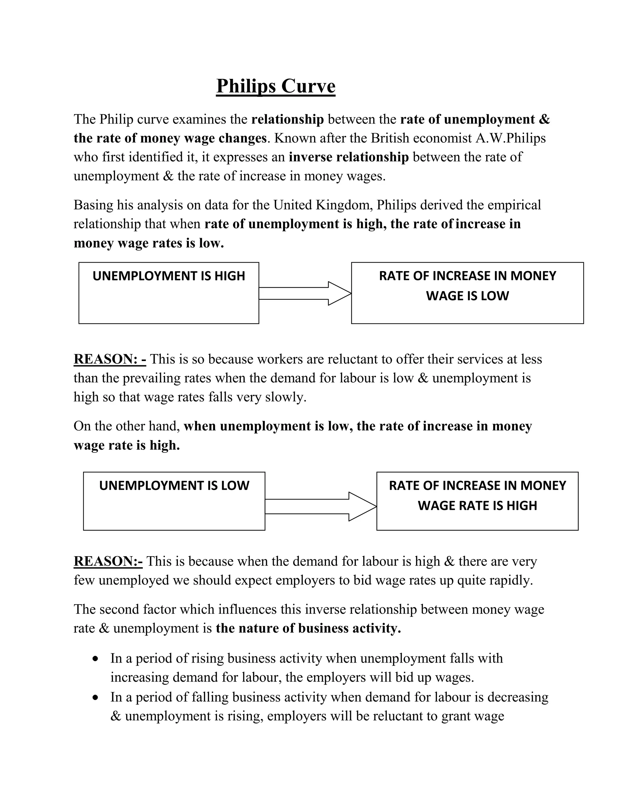
The Philip curve shows an inverse relationship between the rate of unemployment and the rate of change in money wages in the short run. Friedman argued that in the long run, there is no tradeoff between inflation and unemployment - the Philip curve becomes vertical at the natural rate of unemployment, which is the rate where expected and actual inflation are equal. Temporary reductions in unemployment below the natural rate are only possible if inflation rises above expectations, but eventually expectations will adjust and unemployment will return to the natural rate, even as inflation accelerates.

1. Philips Curve
The Philip curve examines the relationship between the rate of unemployment &
the rate of money wage changes. Known after the British economist A.W.Philips
who first identified it, it expresses an inverse relationship between the rate of
unemployment & the rate of increase in money wages.
Basing his analysis on data for the United Kingdom, Philips derived the empirical
relationship that when rate of unemployment is high, the rate of increase in
money wage rates is low.
REASON: - This is so because workers are reluctant to offer their services at less
than the prevailing rates when the demand for labour is low & unemployment is
high so that wage rates falls very slowly.
On the other hand, when unemployment is low, the rate of increase in money
wage rate is high.
REASON:- This is because when the demand for labour is high & there are very
few unemployed we should expect employers to bid wage rates up quite rapidly.
The second factor which influences this inverse relationship between money wage
rate & unemployment is the nature of business activity.
In a period of rising business activity when unemployment falls with
increasing demand for labour, the employers will bid up wages.
In a period of falling business activity when demand for labour is decreasing
& unemployment is rising, employers will be reluctant to grant wage
RATE OF INCREASE IN MONEY
WAGE IS LOW
UNEMPLOYMENT IS HIGH
UNEMPLOYMENT IS LOW RATE OF INCREASE IN MONEY
WAGE RATE IS HIGH

2. increases. Rather they will reduce wages. But workers & unions will be
reluctant to accept wage cuts during g such periods. Consequently,
employers are forced to dismiss workers, thereby leading to high rate of
unemployment.
Thus, when the labour market is depressed, a small reduction in wages would
lead to large increase in unemployment. Philips concluded on the basis of above
arguments that the relation between rate of unemployment & a change of
money wage would be high non-linear when shown on the diagram. Such a
curve is called the Philips curve.
U = UNEMPLOYMENT
W = MONEY WAGE RATE
P = PRICE LEVEL OR INFLATION RATE
0 2 3 4 5
6
-1
5
4
3
2
1
-2
3
2
1
0
M
C
B
A
S
PC
5.5
U
P W
FIGURE: - 1
X
Y

3. Explanation:-
The PC curve in Fig 1relate the %age change in money wage rate on the
vertical axis with the rate of unemployment on horizontal axis. The PC
Curve is known as Philip curve.
The curve is convex to the origin which shows that %age change in money
wag rises with decrease in unemployment rate.
In the figure, when the money wage rate is 2%, the unemployment rate is
3%.But when the money wage rate is high at 4%; the unemployment rate is
low at 2%.
The original Philip curve was an observed statistical relation which was
explained theoretically by Lipsey as resulting from the behavior of labour
market in disequilibrium through excess demand.
Several economists have extended the Philip curve analysis to the trade off
between the rate of unemployment & the rate of change in level of prices or
inflation rate by assuming that prices would change whenever wage rose more
rapidly than labour productivity.
If the rate of increase in money wage is higher then the growth rate of
labour productivity, price will rise & vice versa.
But prices do not rise if labour productivity increases at the same rate as
money wage rate rise.
This trade-off between the inflation & unemployment rate can be
explained with fig 1 where inflation rate (P) is taken on vertical axis
along the rate of change in money wage (W).
Suppose labour productivity rises by 2% per year & if money wage also
increases by 2% , the price level remain constant.
Thus point B on the PC curve corresponding to percentage change in
money wage (M) & unemployment rate of 3% equal 0% inflation rate (P)
on the vertical axis.
The difference between money wage rate & the rate of labour
productivity is inflation rate.

4. Now assume that economy is operating at point B.If now aggregate
demand is increased, this lower the unemployment rate of OT (2%) &
raises the wage rate to OS (4%) per year.
If labour productivity continues to grow at 2% per annum, the price level
will also rise at the rate of 2% per annum at point C.
With the movement of the economy from B to C, unemployment falls to
T (2%).If point B & C are now connected they trace out a Philip curve
PC.
The shape of the PC curve further suggest that when the unemployment rate is less
than 5.5% i.e. left to point A, the demand for labour is more than the supply & this
tend to increase money wage rate. On the other hand, when the unemployment rate
is more than 5.5 % i.e. right to point A, then supply of labour is more than the
demand which tends to lower wage rate. The implication is that the wage rate will
be stable at the unemployment.
It is to noted that PC curve is the „conventional‟ or original downward sloping
Philip curve which show a stable & inverse relation between the rate of
unemployment & the rate of change in wages.

5. FRIEDMAN’S VIEW : THE LONG RUN PHILIP CURVE
Economist have criticized & in certain cases modified the Philip curve. They argue
that the Philip curve relate to short run & it does not remain stable. It shifts with
changes in expectations of inflation. In long-run there is no trade-off between
inflation & unemployment. These views have been expounded by Friedman &
Phelps in what has come to be known as the “accelerationist” or the “adaptive
expectations” hypothesis.
According to Friedman, there is no need to assume a stable downward sloping
Philip curve to explain the trade-off between inflation & unemployment. In fact,
this relation is a short-run phenomenon. But there are certain variable which cause
the Philip curve to shift over time & the most important of them is the expected
rate of inflation. So long as there is discrepancy between the expected rate & the
actual rate of inflation, the downward sloping Philip curve will be found. But when
this discrepancy is removed over the long run, the Philip curve becomes vertical.
In order to explain this, Friedman introduces the concept of the natural rate of
unemployment. It represents the rate of unemployment at which the economy
normally settles because of its structural imperfections. It is the unemployment rate
below which the inflation rate increases & above which the inflation rate
decreases.
At this rate, there is neither a tendency for the inflation rate to increase or decrease.
Thus the natural rate of unemployment is defined as the rate of unemployment at
which the actual rate of inflation equals the expected rate of inflation. It is thus an
equilibrium rate of unemployment towards which the economy moves in the long
run.
In the long run, the Philip curve is a vertical line at the natural rate of
unemployment. This is the natural or equilibrium unemployment rate is not fixed
for all times. Rather, it is determined by a number of structural characteristics of
the labor & commodity market within the economy. These may be minimum wage
laws, inadequate employment information, deficiencies in manpower training,
costs of labour mobility, & other market imperfections. But what causes the Philip
curve to shift over time is the expected rate of inflation. This refers to the extent
the labour correctly forecasts inflation & can adjust wages to the forecast.

6. Suppose the economy is experiencing a mild rate of inflation of 2% & a
natural rate of unemployment (N) of 3%.
At point A on the short-run Philip curve SPC1 in fig2 people expect this rate
of inflation in the future.
Now assume that the government adopts a monetary-fiscal programme to
raise aggregate demand in order to lower unemployment from 3% to 2%.
The increase in aggregate demand will raise the rate of inflation to 4%
consistent with the unemployment rate 2%.
SPC 1
SPC 2
SPC 3
LPC
0 1 2 3
4
6
E
C
A
D
B
F8
2
UNEMPLOYMENT (%)
I
N
F
L
A
T
I
O
N
%
FIGURE: - 2
X
Y

7. When the actual inflation rate (4%) is greater than the expected inflation rate
(2%), the economy moves from point A to B along the SPC1 curve & the
unemployment rate temporarily falls to 2%.
This is achieved because the labour has been deceived. It expected the
inflation rate of 2% & based their wage demand on this rate. But the workers
eventually begin to realize that the actual rate of inflation is 4% which now
become their expected rate of inflation.
Once this happens the short run Philip curve SPC1 shifts to the right to
SPC2.Now workers demand increases in money wages to meet the higher
expected rate of inflation of 4%.They demand higher wages because, they
consider the present money wages to be inadequate in real terms. In others
words, they want to keep up with the higher prices & to eliminate fall in real
wages.
As a result, real labour costs will rise, firms will discharge workers &
unemployment will raise form B (2%) to C (3%) with the shifting of the
SPC1 curve to SPC2.
At point C, the natural rate of unemployment is re-established at a higher
rate of both the actual & expected inflation (4%).
If the government is determined to maintain the level of unemployment at
2%, it can do so only at the cost of high rates of inflation.
From point C, unemployment once again can be reduced to 2% via increase
in its aggregate demand along the SPC2 curve until we arrive at point D.
With 2% unemployment & 6% inflation at point D, the expected rate of
inflation for workers is 4%. As soon as they adjust their expectations to the
new situation of 6% inflation, the short-run Philip curve shifts up again to
SPC3, & the unemployment will rise back to its natural level of 3% at point
E.
If point A, C, &E are connected, they trace out a vertical long run Philip
Curve LPC at the natural rate of unemployment. On this curve, there is no
trade-off between unemployment & inflation.
Rather, any one of several rates of inflation at point A, C &E is compatible
with the natural unemployment rate of 3%.
Any reduction in unemployment rate below its natural rate will be associated
with an accelerating & ultimately explosive inflation. But this is only

8. possible temporarily so long as workers overestimate or underestimate the
inflation rate.
In long-run, the economy is bound to establish at the natural unemployment
rate.
There is therefore no trade-off between unemployment & inflation except in the
short-run. This is because inflationary expectations are revised according to what
has happened to inflation in the post. So when the actual rate of inflation, say, rises
to 4%, workers continue to expect 2% inflation for a while & only in the long run
they revise their expectation upward to 4%. Since they adapt themselves to the
expectations hypothesis. According to this hypothesis, the expected rate of
inflation always lags behind the actual rate. But if actual rate remains constant, the
expected rate would ultimately become equal to it.
This leads to the conclusion that a short-run trade-off exists between
unemployment & inflation, but there is no long trade-off between the two unless a
continuously rising inflation rate is tolerated.

9. CRITICISM
The accelerationist hypothesis of Friedman has been criticized on the following
grounds:-
1. The vertical long-run Philips Curve relates to steady rate of inflation. But
this is not a correct view because the economy is always passing through a
series of disequilibrium position with little tendency to approach a steady
state. In such a situation, expectation may be disappointed year after year.
2. Friedman does not give a new theory of how expectations are formed that
would be free from theoretical & statistical bias. This makes his position
unclear.
3. In one of his writing Friedman himself accepts the possibility that the long-
run Philips curve might not just be vertical, but could be positively sloped
with increasing dose of inflation leading to increasing unemployment.
4. Some economist have argued that wage rate have not increased at a high rate
of unemployment.
5. It is believed that workers have a money illusion. They are more concerned
with the increase in the money wage rates than real wage rates.
6. Some economist regards the natural rate of employment as a mere
abstraction because Friedman has not tried to define in concrete terms.