Downloaded 120 times
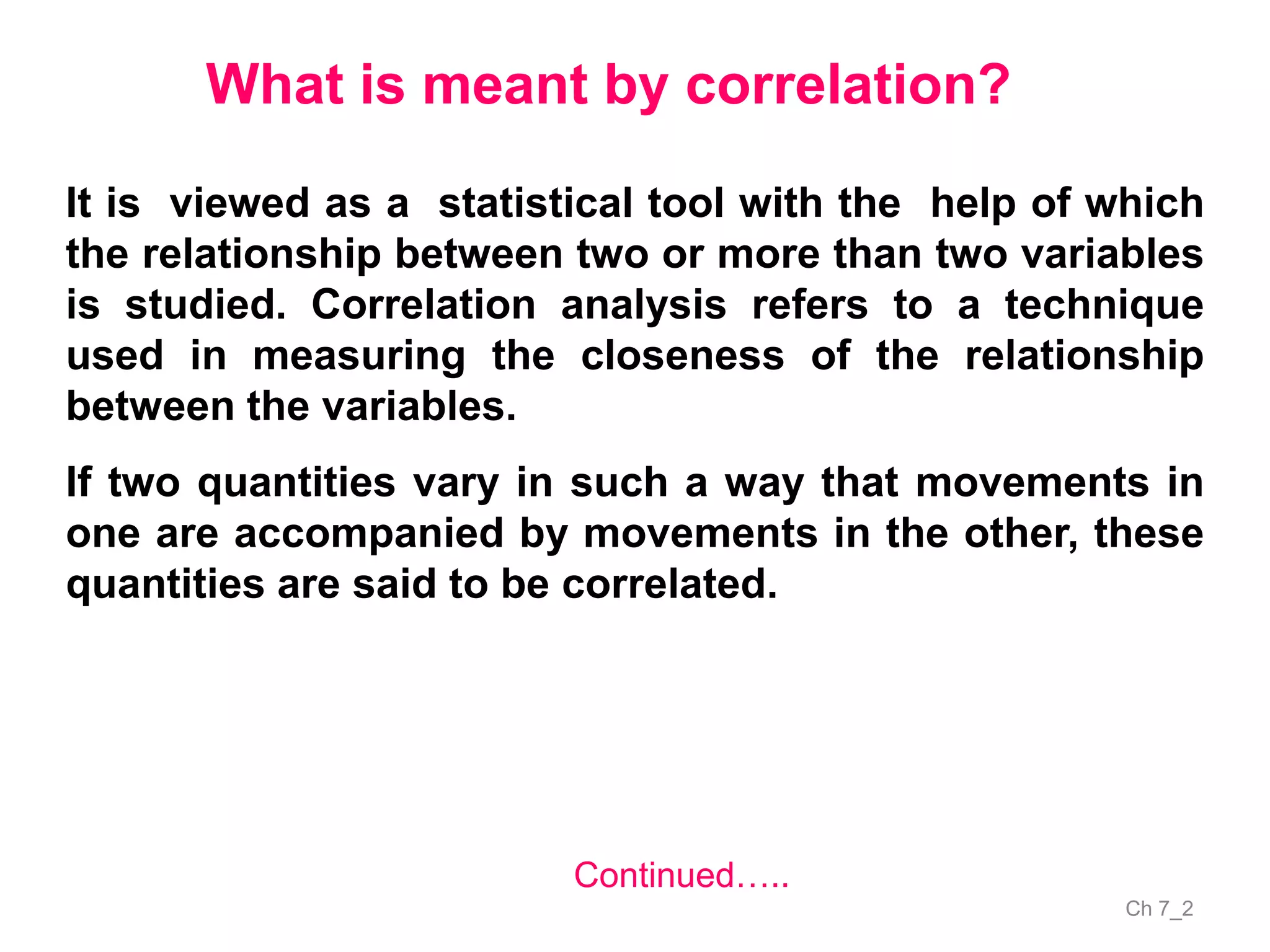
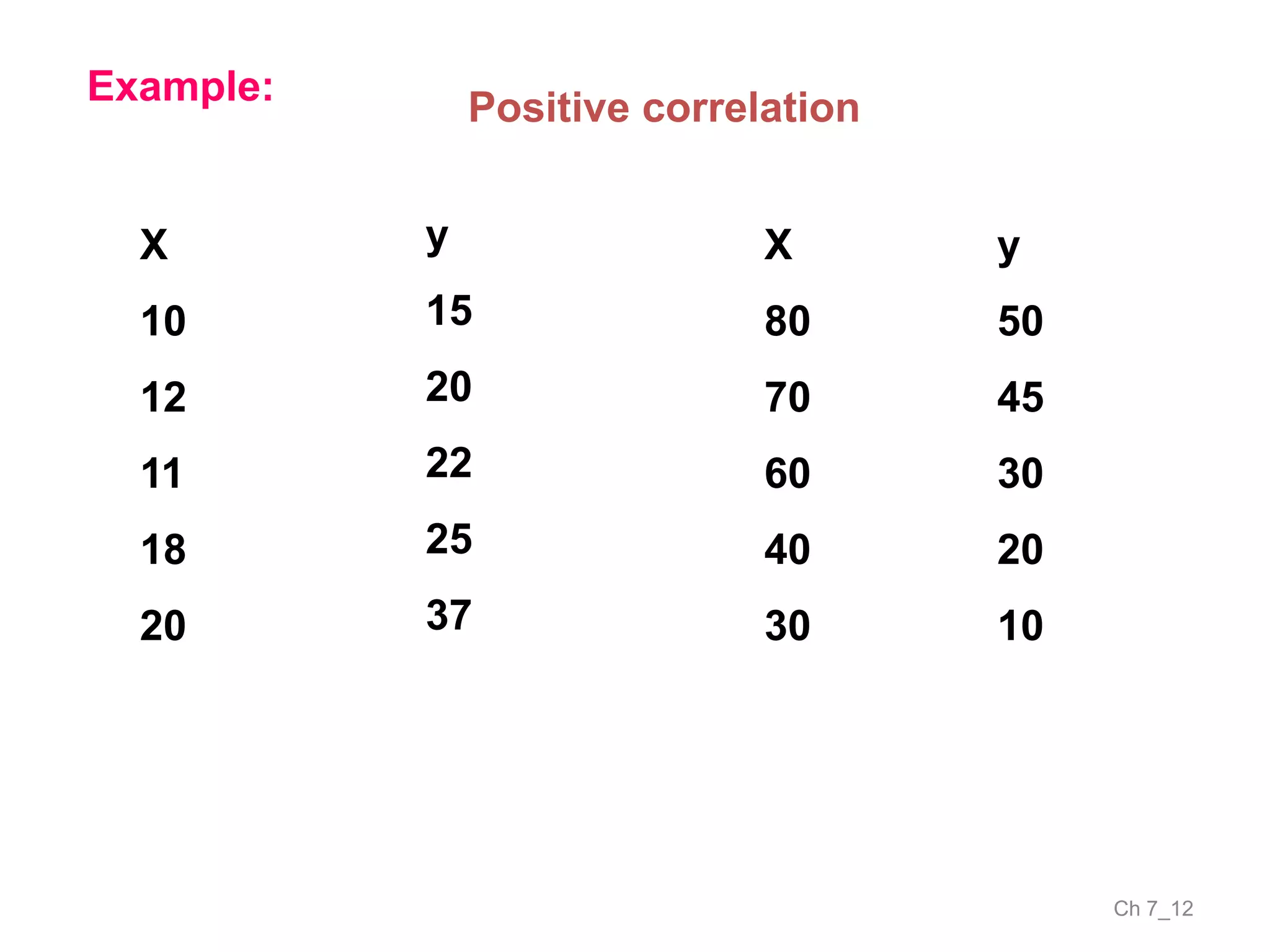
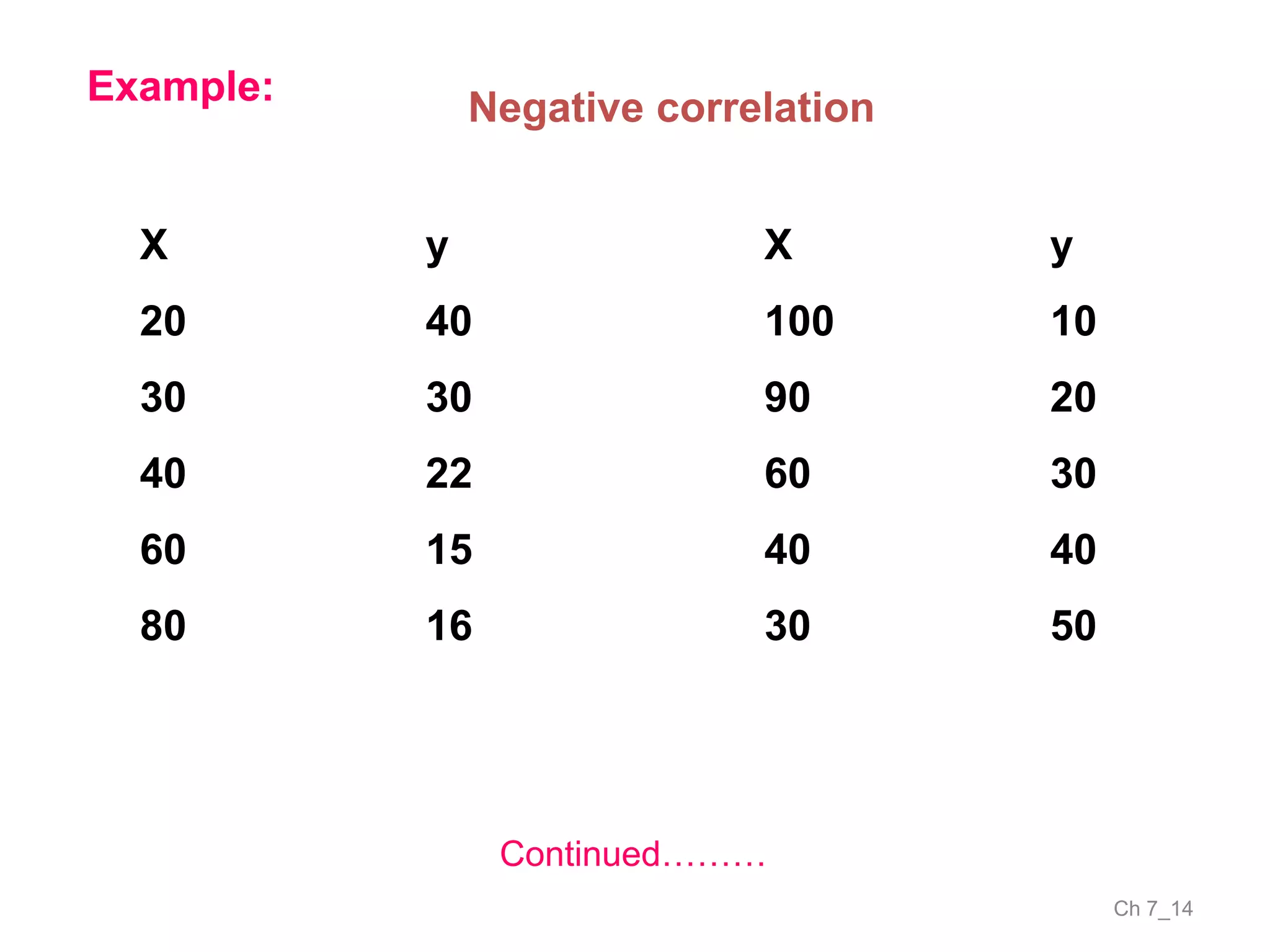
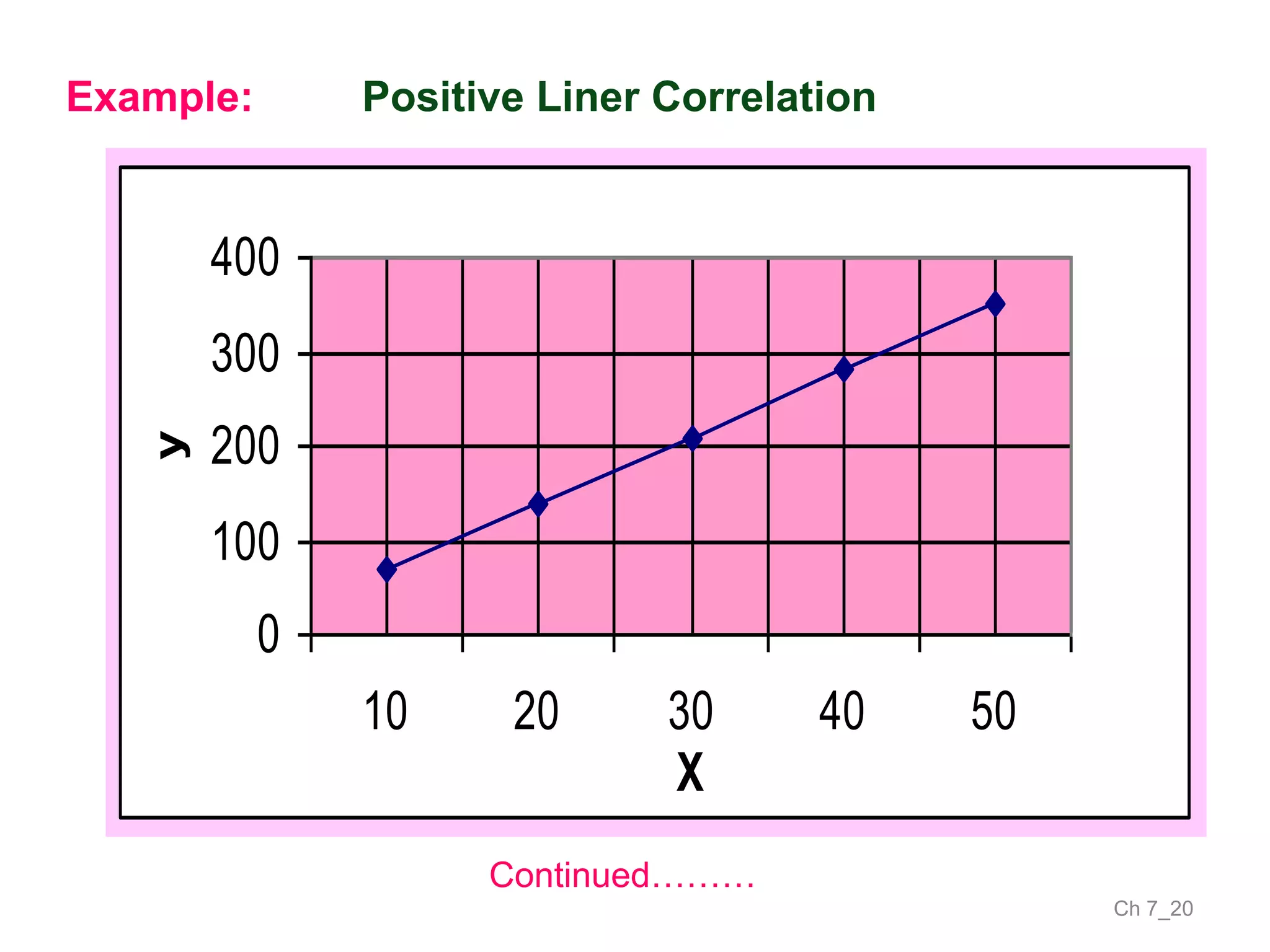
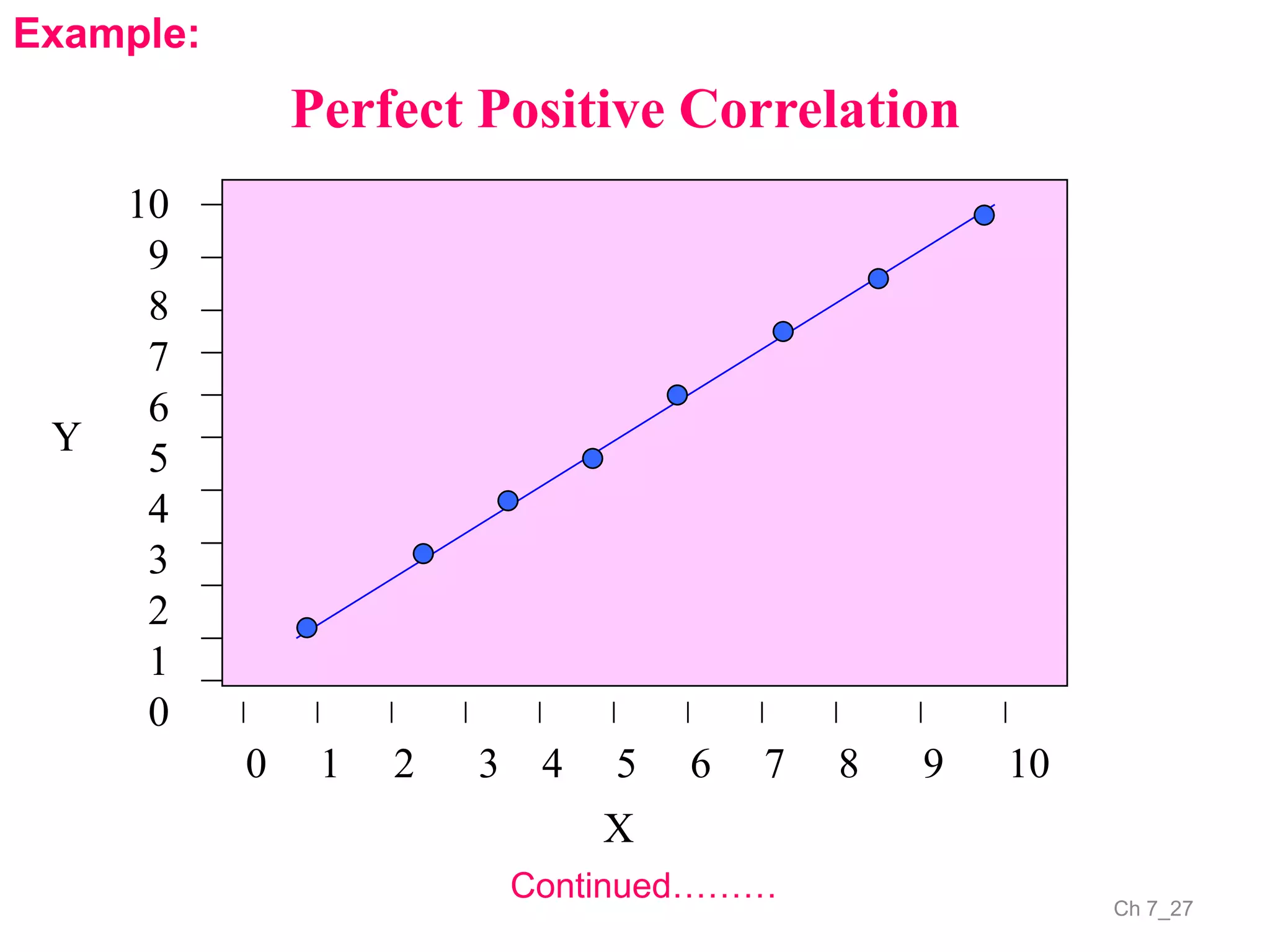
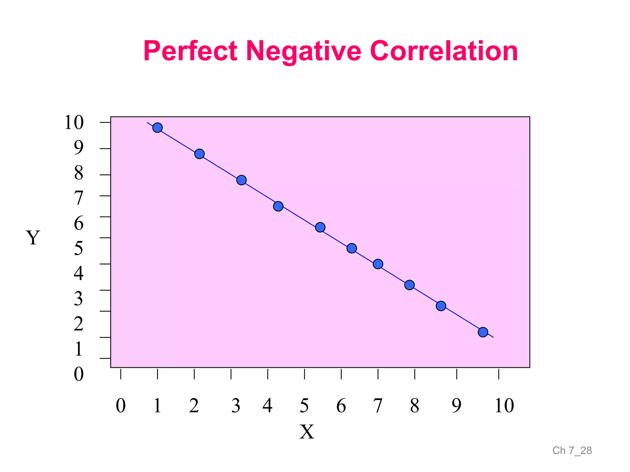
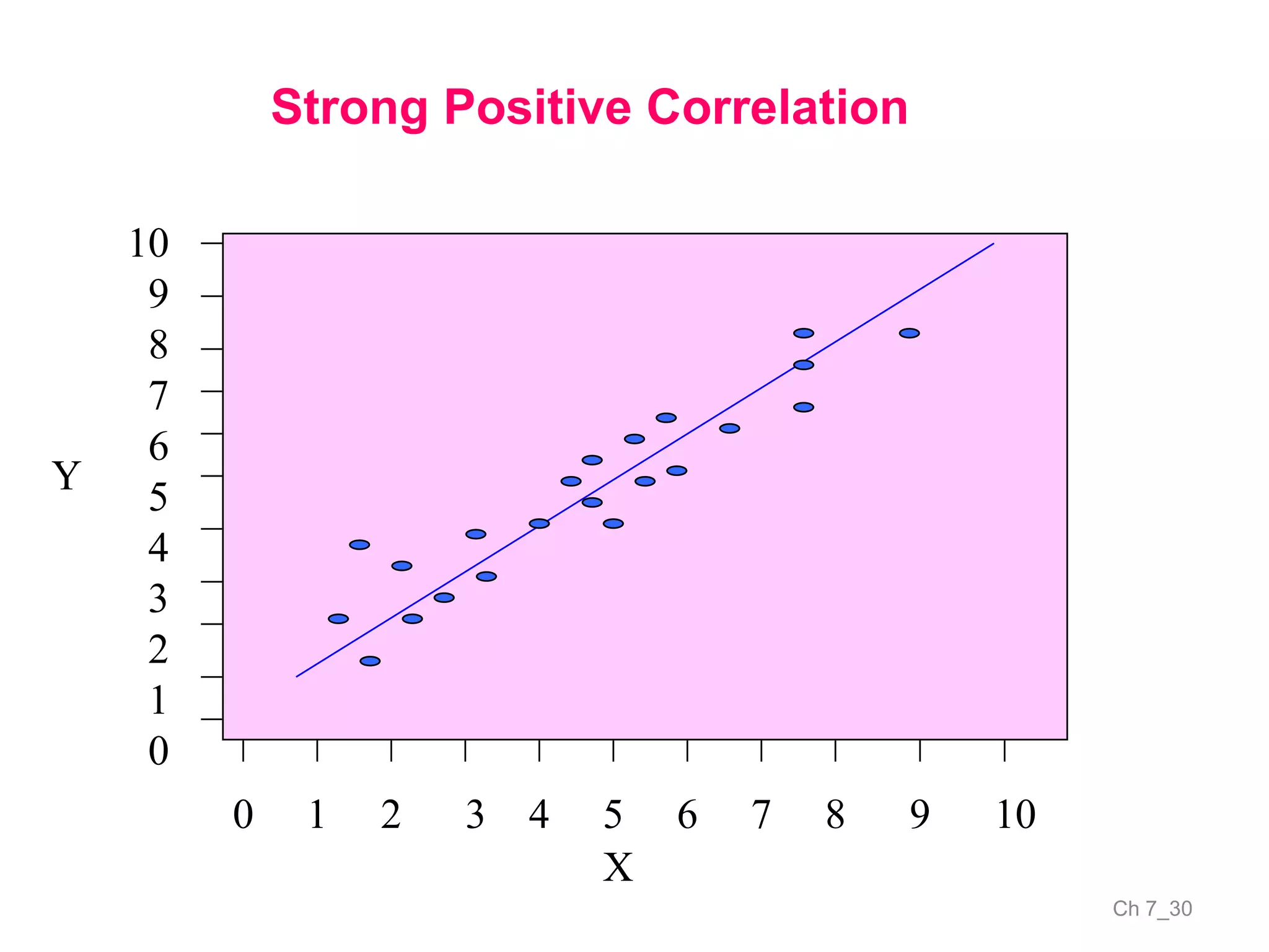
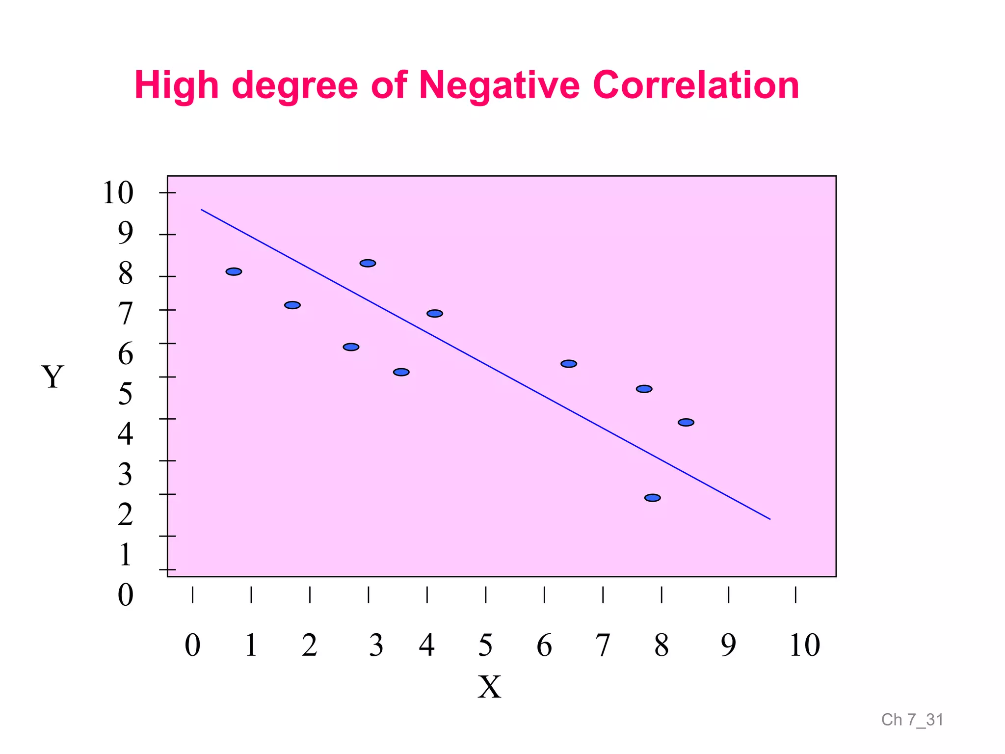
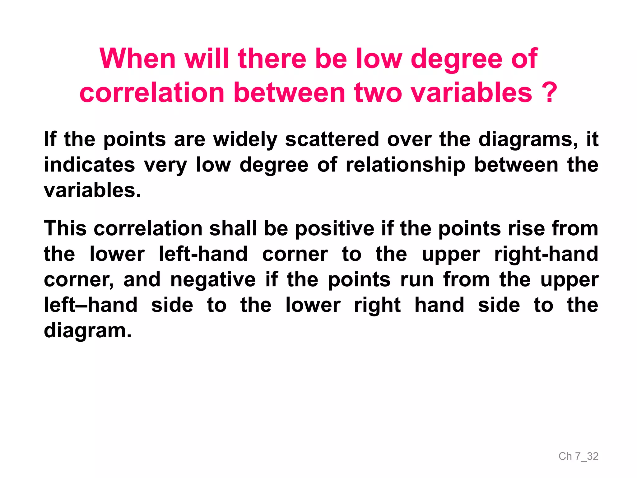
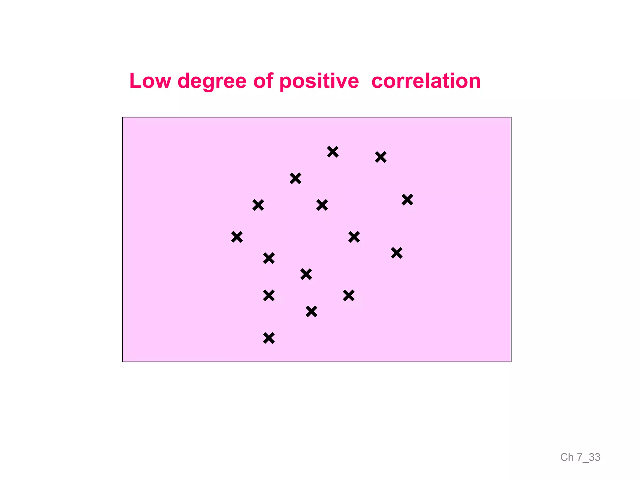
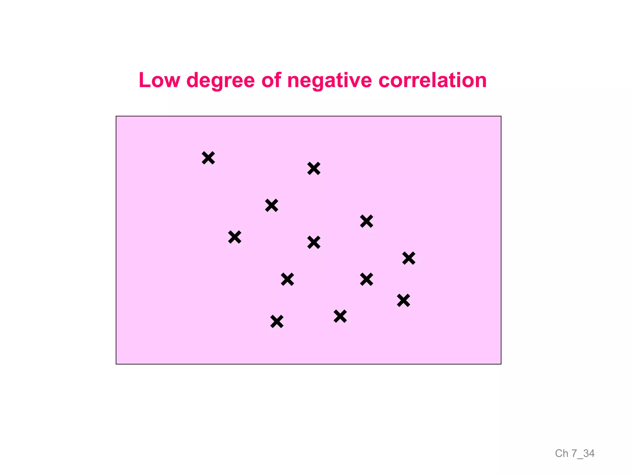
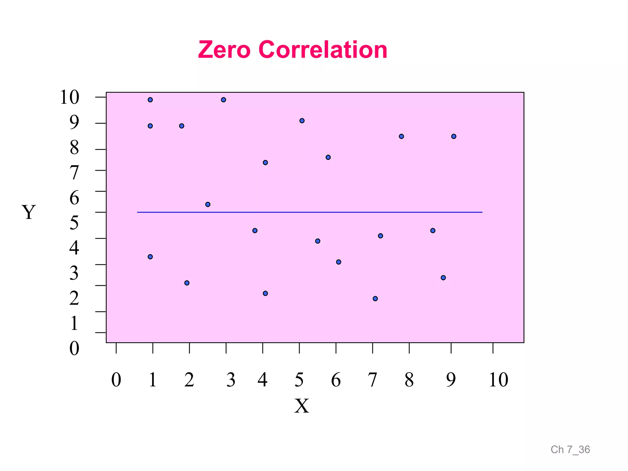
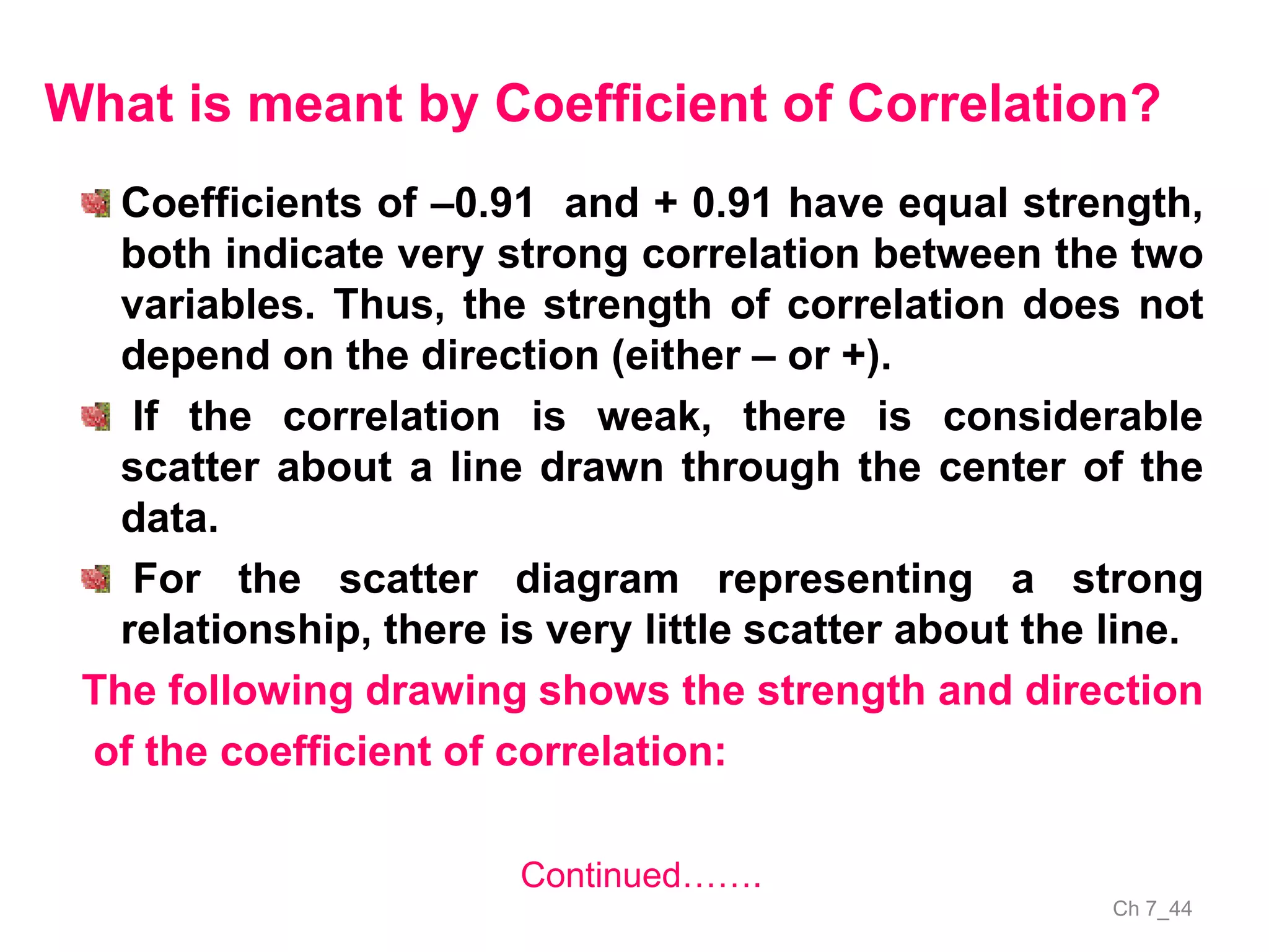
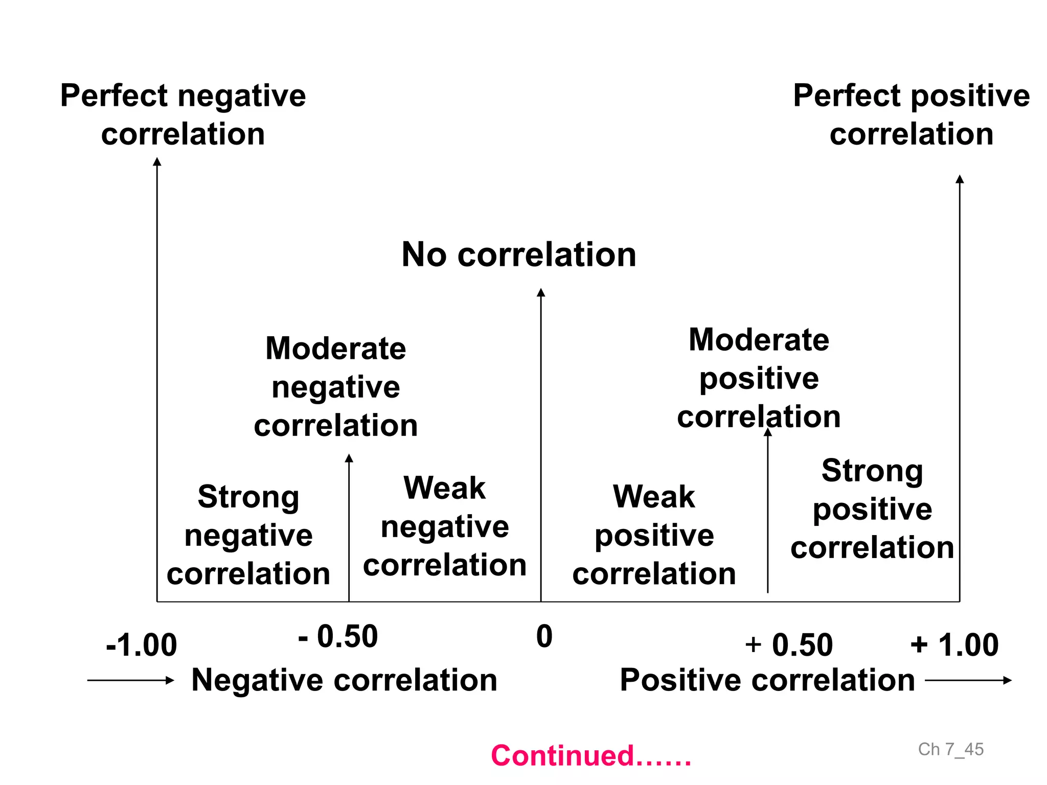
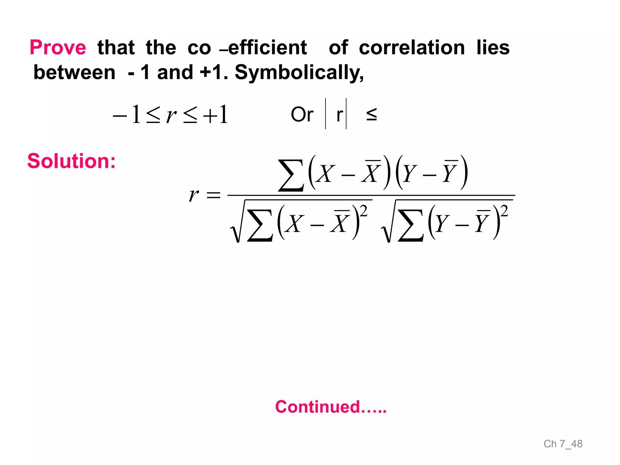
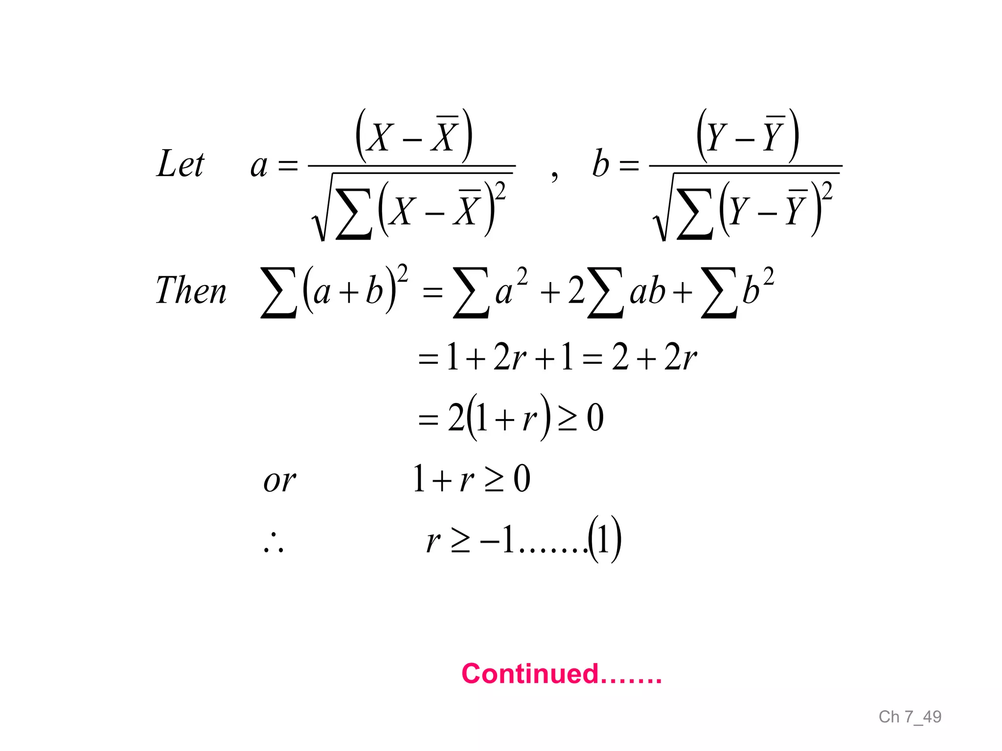
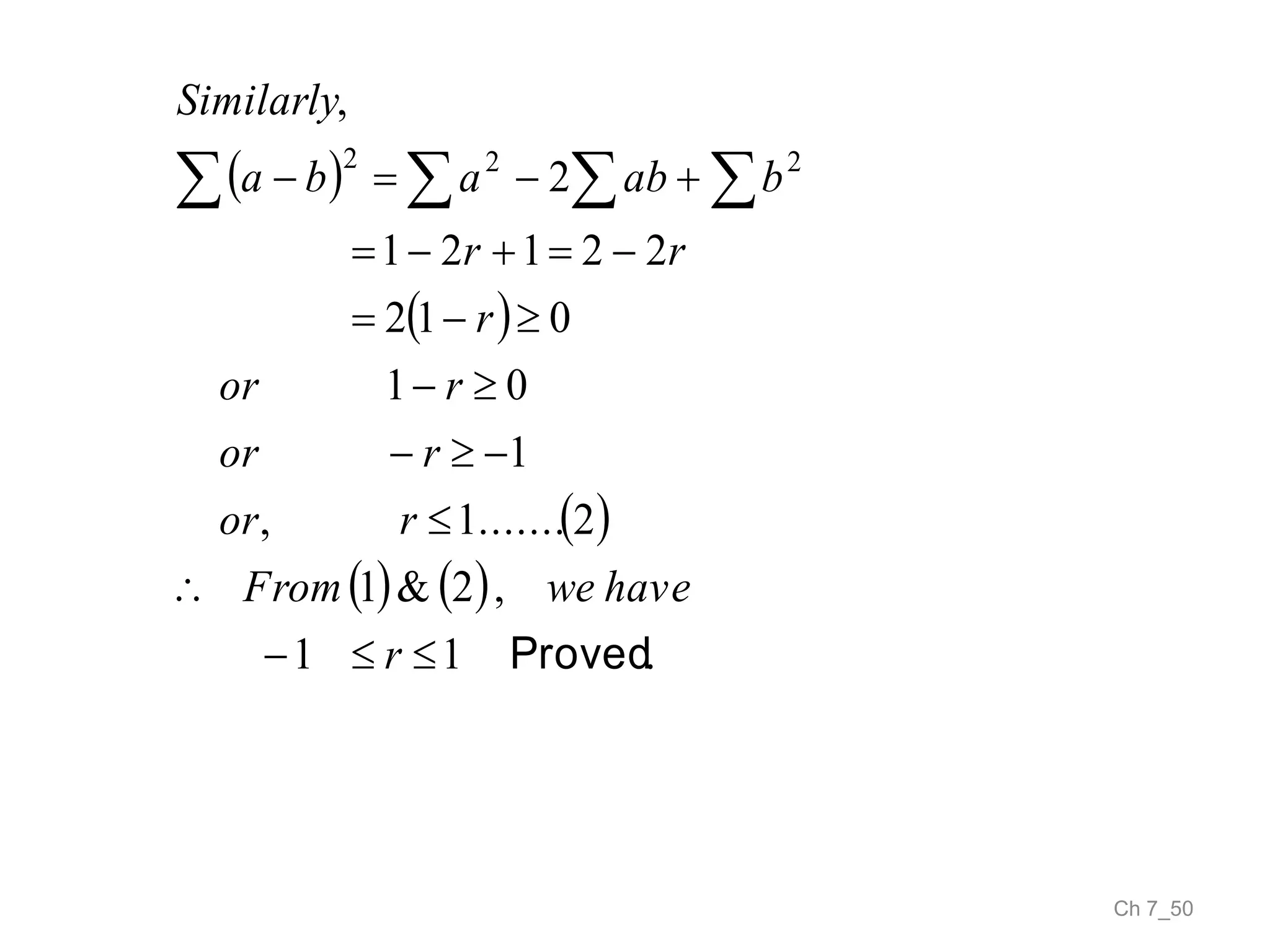
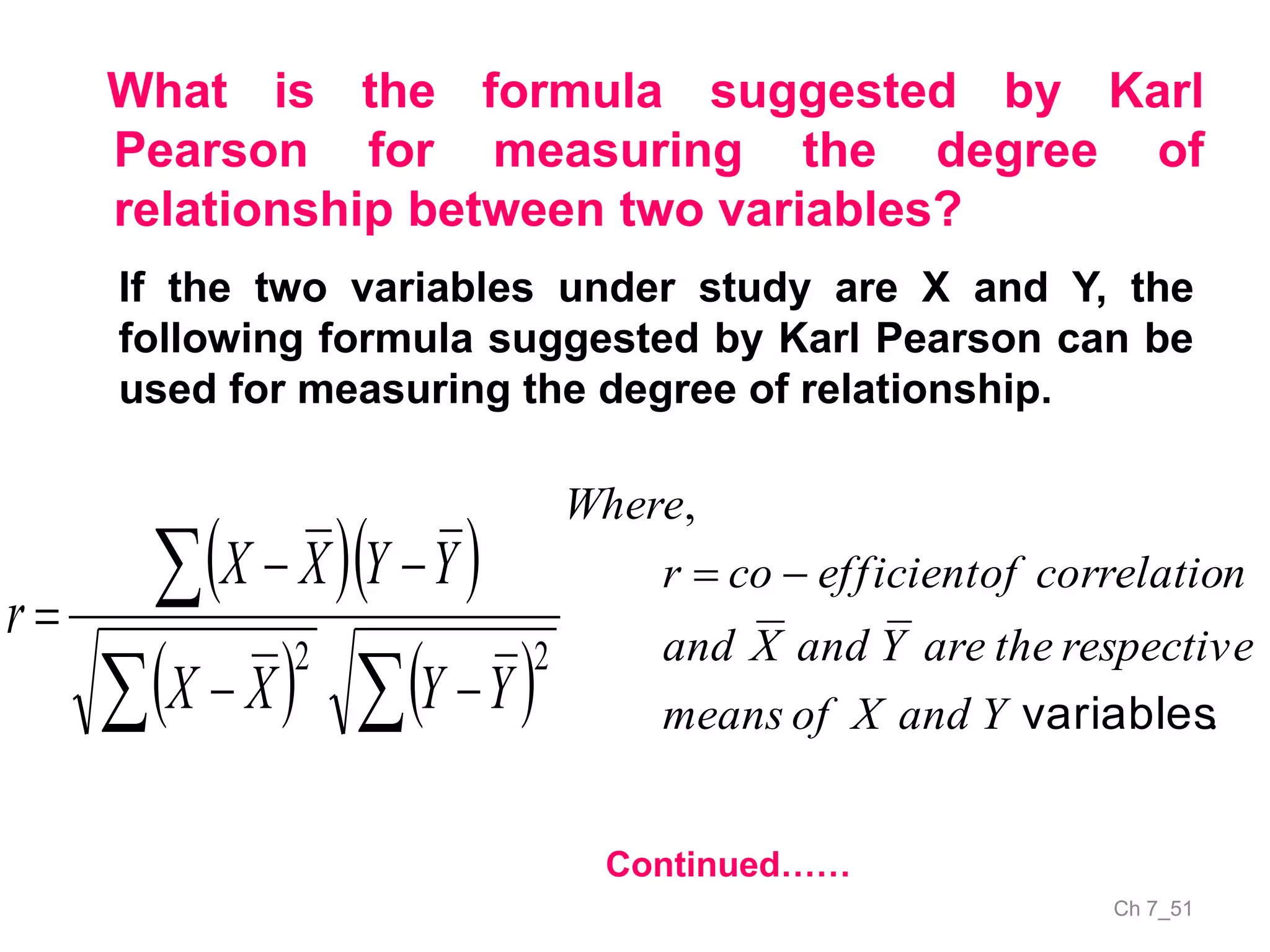
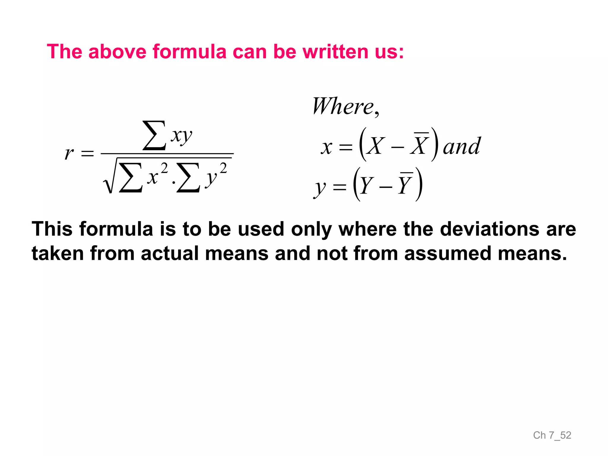
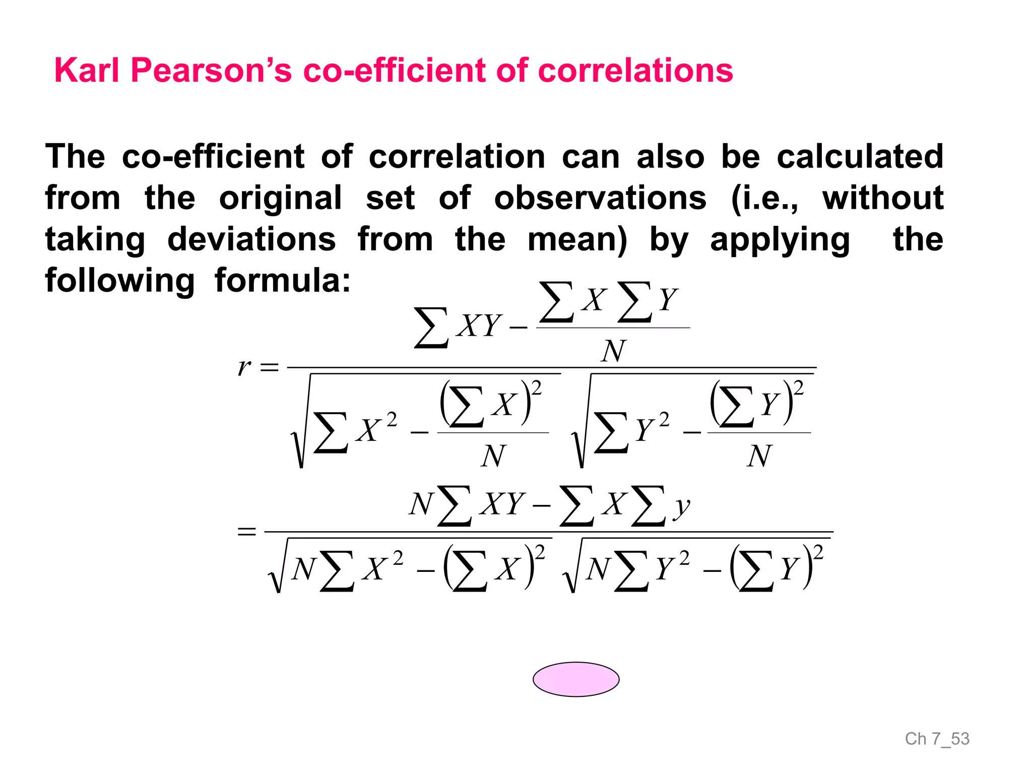
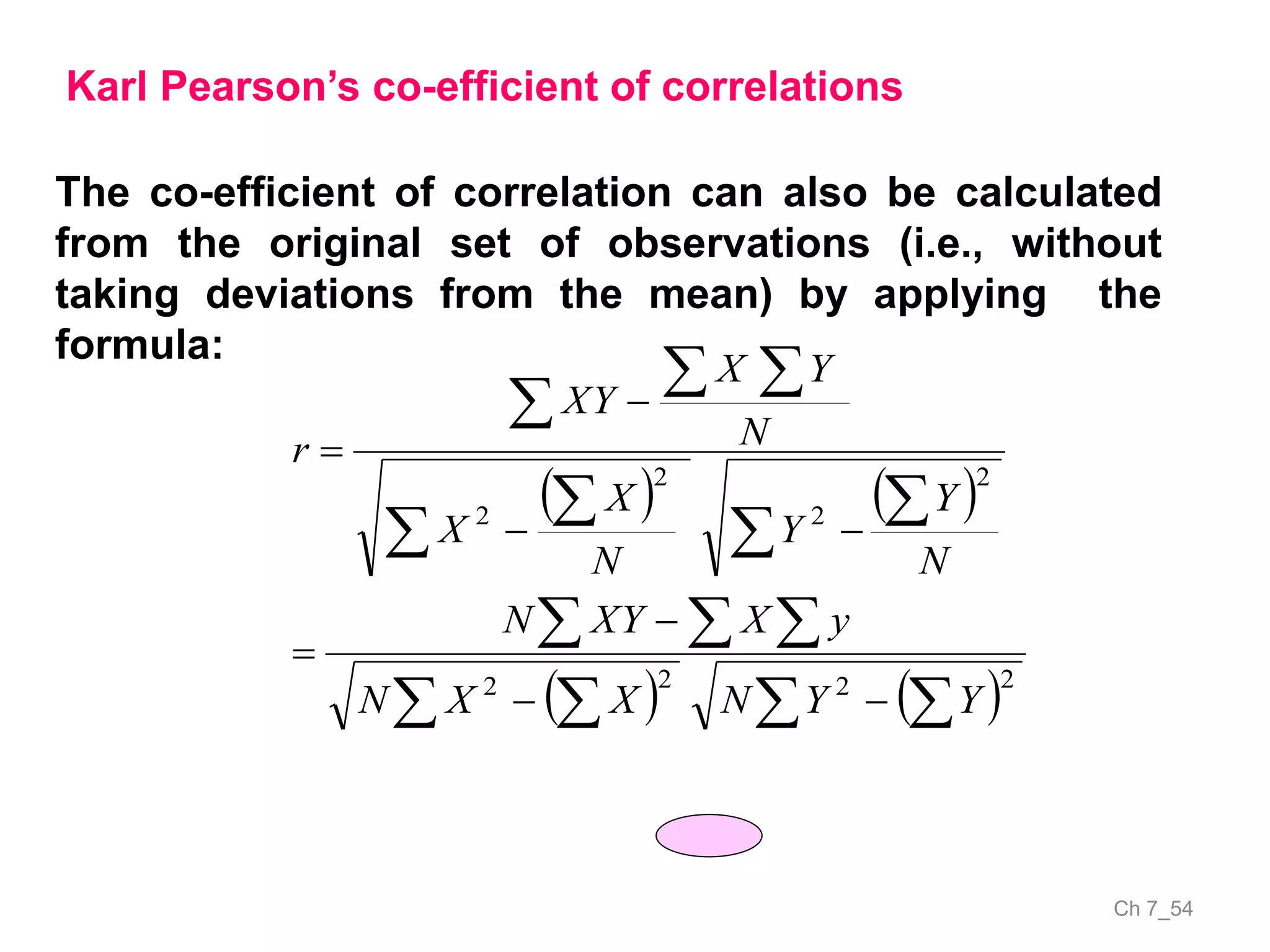
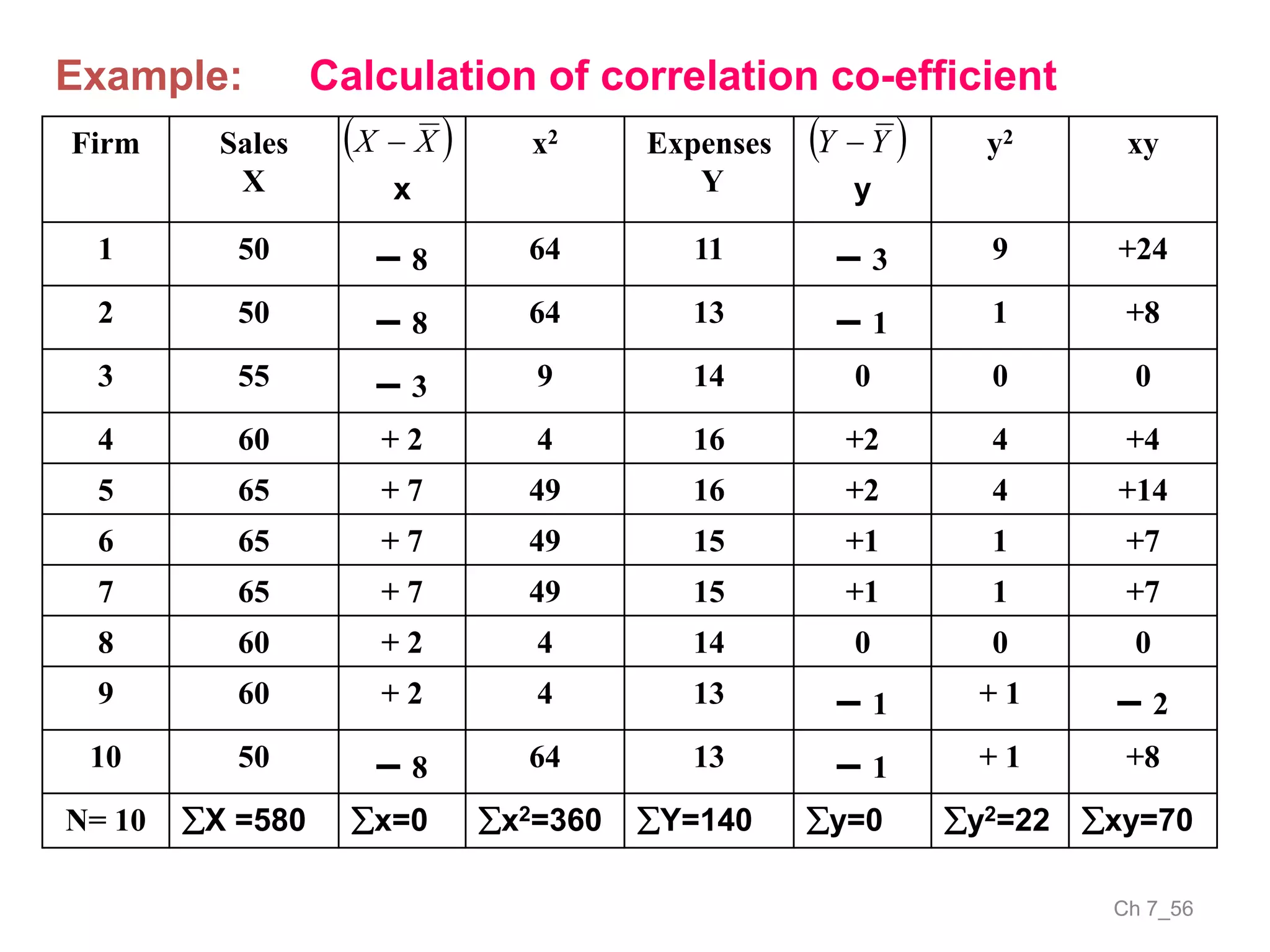
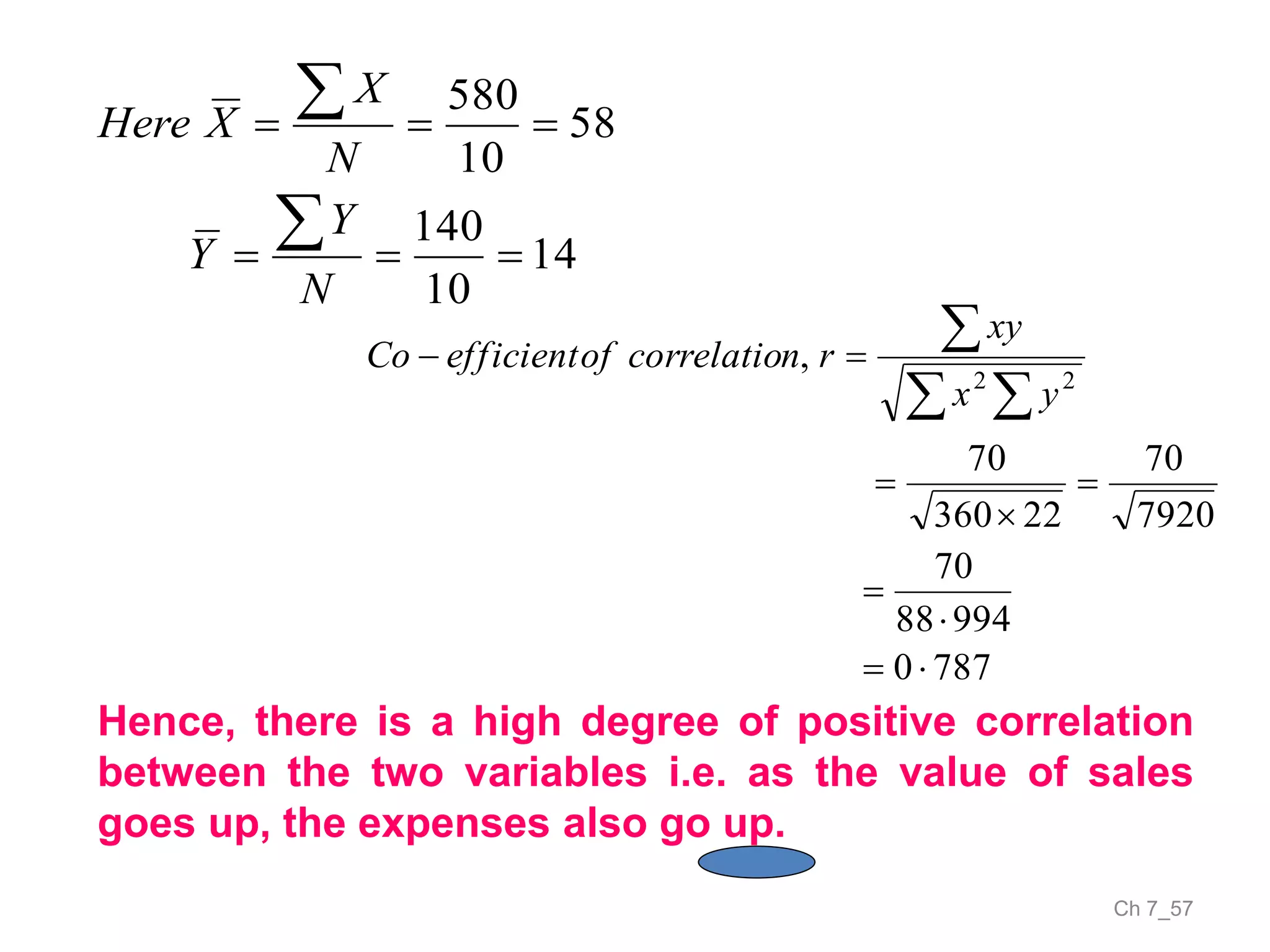
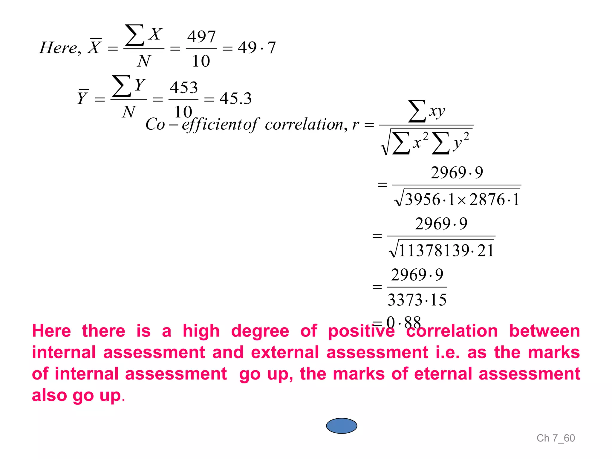
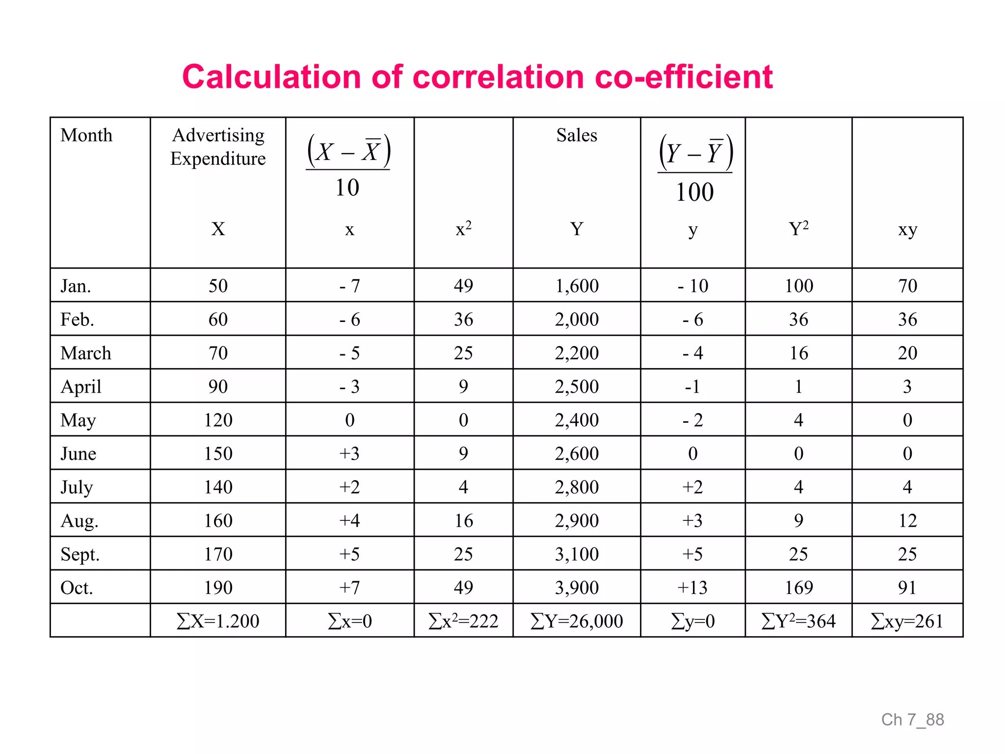
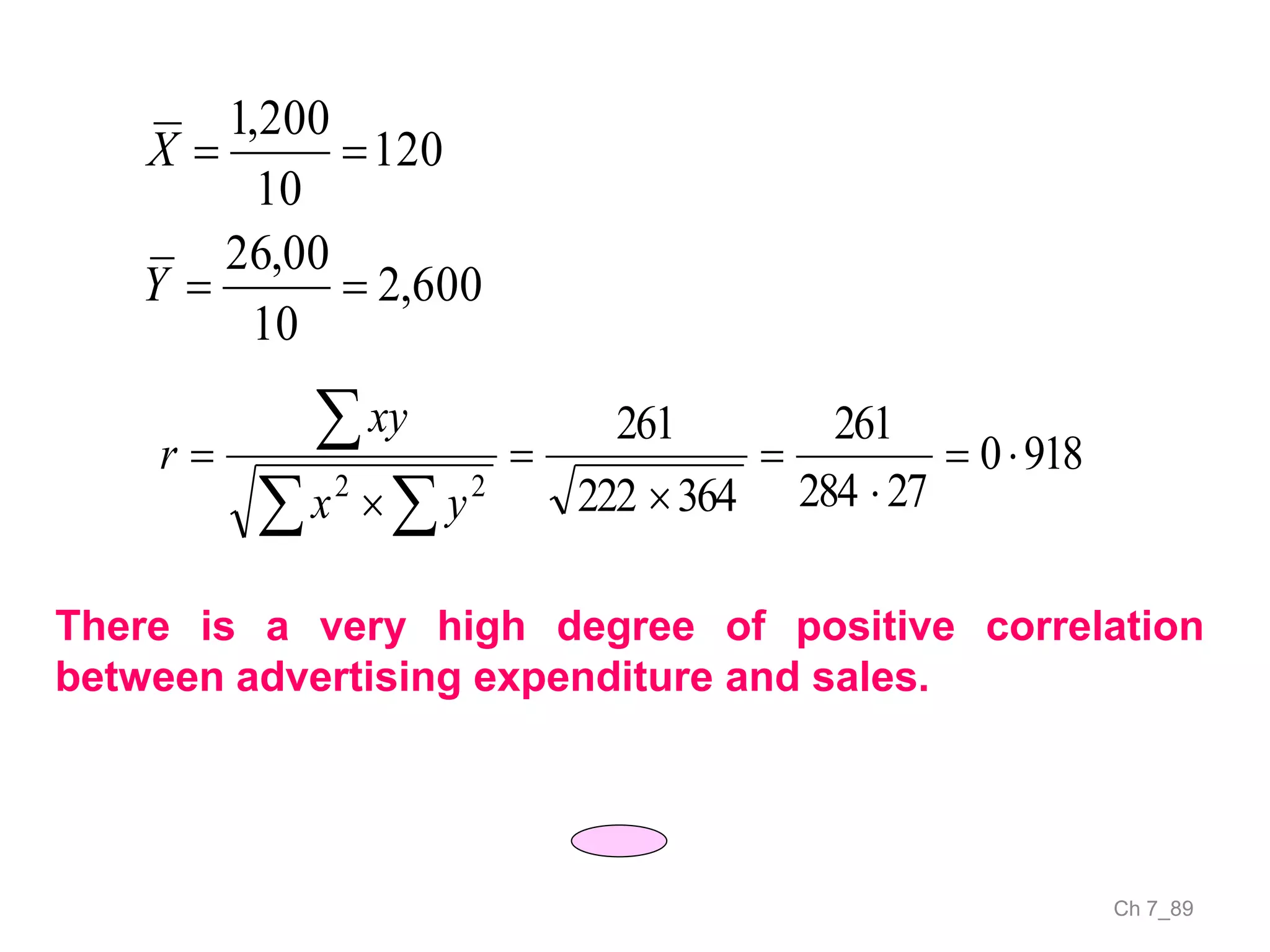

The document discusses correlation and the coefficient of correlation. It defines correlation as a statistical tool used to study the relationship between two or more variables. The coefficient of correlation (r) is a measure of the strength and direction of the linear relationship between variables. r can range from -1 to 1, where -1 is perfect negative correlation, 0 is no correlation, and 1 is perfect positive correlation. A scatter diagram can be used to visually depict the relationship between variables and provide an initial assessment of correlation.


![correlation-ppt [Autosaved].pptx statistics in BBA from parul University](https://cdn.slidesharecdn.com/ss_thumbnails/correlation-pptautosaved-240401173254-81d64a83-thumbnail.jpg?width=640&height=640&fit=bounds)