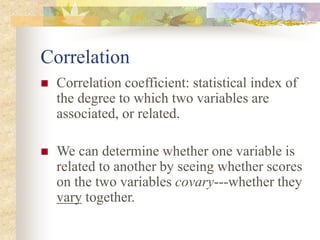
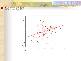
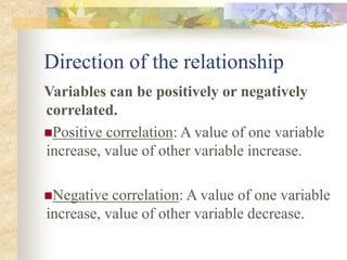
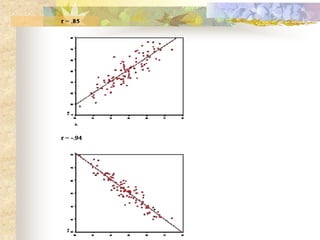
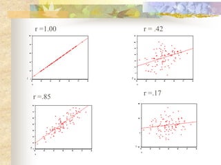
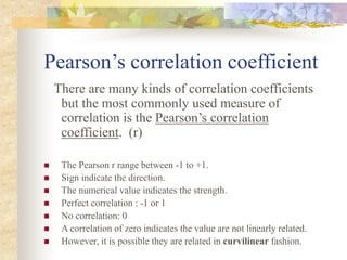
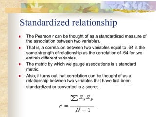
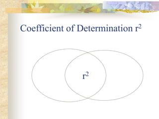
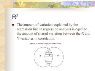
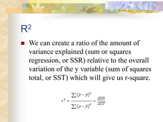
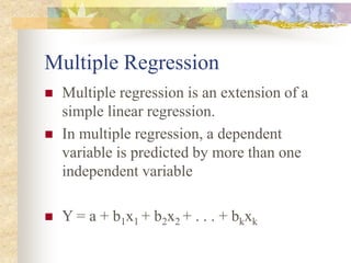
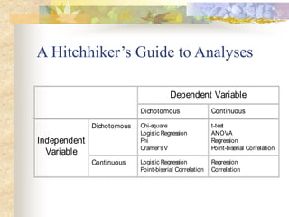
This document provides an overview of correlation and linear regression analysis. It defines correlation as a statistical measure of the relationship between two variables. Pearson's correlation coefficient (r) ranges from -1 to 1, with values farther from 0 indicating a stronger linear relationship. Positive values indicate an increasing relationship, while negative values indicate a decreasing relationship. The coefficient of determination (r2) represents the proportion of shared variance between variables. While correlation indicates linear association, it does not imply causation. Multiple regression allows predicting a continuous dependent variable from two or more independent variables.

1. Review
I am examining differences in the mean between groups
How many independent variables?
One More than one
How many groups?
Two More than two
? ? ?

2. Differences or Relationships?
I am examining
relationships
between variables
I am examining
differences between
groups
T-test, ANOVA Correlation,
Regression Analysis

3. Example of Correlation
Is there an association between:
 Children’s IQ and Parents’ IQ
 Degree of social trust and number of membership
in voluntary association ?
 Urban growth and air quality violations?
 GRA funding and number of publication by Ph.D.
students
 Number of police patrol and number of crime
 Grade on exam and time on exam

4. Correlation
 Correlation coefficient: statistical index of
the degree to which two variables are
associated, or related.
 We can determine whether one variable is
related to another by seeing whether scores
on the two variables covary---whether they
vary together.

5. Scatterplot
 The relationship between any two variables
can be portrayed graphically on an x- and
y- axis.
 Each subject i1 has (x1, y1). When score s
for an entire sample are plotted, the result
is called scatter plot.

6.  Scatterplot

7. Direction of the relationship
Variables can be positively or negatively
correlated.
Positive correlation: A value of one variable
increase, value of other variable increase.
Negative correlation: A value of one variable
increase, value of other variable decrease.

9. Strength of the relationship
The magnitude of correlation:
 Indicated by its numerical value
 ignoring the sign
 expresses the strength of the linear
relationship between the variables.

10. r =1.00
r =.17
r = .42
r =.85

11. Pearson’s correlation coefficient
There are many kinds of correlation coefficients
but the most commonly used measure of
correlation is the Pearson’s correlation
coefficient. (r)
 The Pearson r range between -1 to +1.
 Sign indicate the direction.
 The numerical value indicates the strength.
 Perfect correlation : -1 or 1
 No correlation: 0
 A correlation of zero indicates the value are not linearly related.
 However, it is possible they are related in curvilinear fashion.

12. Standardized relationship
 The Pearson r can be thought of as a standardized measure of
the association between two variables.
 That is, a correlation between two variables equal to .64 is the
same strength of relationship as the correlation of .64 for two
entirely different variables.
 The metric by which we gauge associations is a standard
metric.
 Also, it turns out that correlation can be thought of as a
relationship between two variables that have first been
standardized or converted to z scores.

13. Correlation Represents
a Linear Relationship
 Correlation involves a linear relationship.
 "Linear" refers to the fact that, when we graph our
two variables, and there is a correlation, we get a
line of points.
 Correlation tells you how much two variables are
linearly related, not necessarily how much they are
related in general.
 There are some cases that two variables may have
a strong, or even perfect, relationship, yet the
relationship is not at all linear. In these cases, the
correlation coefficient might be zero.

15. Coefficient of Determination r2
 The percentage of shared variance is represented
by the square of the correlation coefficient, r2 .
 Variance indicates the amount of variability in a
set of data.
 If the two variables are correlated, that means that
we can account for some of the variance in one
variable by the other variable.

16. Coefficient of Determination r2
r2

17. Statistical significance of r
 A correlation coefficient calculated on a sample is
statistically significant if it has a very probability
of being zero in the population.
 In other words, to test r for significance, we test
the null hypothesis that, in the population the
correlation is zero by computing a t statistic.
 Ho: r = 0
 HA: r = 0

18. Some consideration in
interpreting correlation
1. Correlation represents a linear relations.
 Correlation tells you how much two variables are
linearly related, not necessarily how much they
are related in general.
 There are some cases that two variables may
have a strong perfect relationship but not linear.
For example, there can be a curvilinear
relationship.

19. Some consideration in
interpreting correlation
2. Restricted range (Slide: Truncated)
 Correlation can be deceiving if the full
information about each of the variable is not
available. A correlation between two variable is
smaller if the range of one or both variables is
truncated.
 Because the full variation of one variables is not
available, there is not enough information to see
the two variables covary together.

20. Some consideration in
interpreting correlation
3. Outliers
 Outliers are scores that are so obviously deviant
from the remainder of the data.
 On-line outliers ---- artificially inflate the
correlation coefficient.
 Off-line outliers --- artificially deflate the
correlation coefficient

21. On-line outlier
 An outlier which falls near where the regression
line would normally fall would necessarily
increase the size of the correlation coefficient, as
seen below.
 r = .457

22. Off-line outliers
 An outlier that falls some distance away from the
original regression line would decrease the size of
the correlation coefficient, as seen below:
 r = .336

23. Correlation and Causation
 Two things that go together may not necessarily
mean that there is a causation.
 One variable can be strongly related to another,
yet not cause it. Correlation does not imply
causality.
 When there is a correlation between X and Y.
 Does X cause Y or Y cause X, or both?
 Or is there a third variable Z causing both X and
Y , and therefore, X and Y are correlated?

24. SPSS Demo

25. Simple Linear Regression
 One objective of simple linear regression is
to predict a person’s score on a dependent
variable from knowledge of their score on
an independent variable.
 It is also used to examine the degree of
linear relationship between an independent
variable and a dependent variable.

26. Example of Linear Regression
 Predict “productivity” of factory workers
based on the “Test of Assembly Speed”
score.
 Predict “GPA” of college students based on
the “SAT” score.
 Examine the linear relationship between
“Blood cholesterol” and “fat intake”.

27. Prediction
 A perfect correlation between two variables produces a
line when plotted in a bivariate scatterplot
 In this figure, every increase of the value of X is
associated with an increase in Y without any exceptions.
If we wanted to predict values of Y based on a certain
value of X, we would have no problem in doing so with
this figure. A value of 2 for X should be associated with a
value of 10 on the Y variable, as indicated by this graph.

28. Error of Prediction:
“Unexplained Variance”
 Usually, prediction won't be so perfect. Most
often, not all the points will fall perfectly on the
line. There will be some error in the prediction.
 For each value of X, we know the approximate
value of Y but not the exact value.

29. Unexplained Variance
 We can look at how much each point falls off the line by drawing a
little line straight from the point to the line as shown below.
 If we wanted to summarize how much error in prediction we had
overall, we could sum up the distances (or deviations) represented by
all those little lines.
 The middle line is called the regression line.

30. The Regression Equation
 The regression equation is simply a
mathematical equation for a line. It is the
equation that describes the regression line.
In algebra, we represent the equation for a
line with something like this:
y = a + bx

31. Sum of Squares Residual
 Summing up the deviations of the points gives us an
overall idea of how much error in prediction there is.
 Unfortunately, this method does not work very well.
 If we choose a line that goes exactly through the middle
of the points, about half of the points that fall off of the
line should be below the line and about half should be
above. Some of the deviations will be negative and some
will be positive, and, thus the sum of all of them will
equal 0.

32. Sum of Squares Residual
 The (imaginary) scores that fall exactly on the
regression line are called the predicted scores,
and there is a predicted score for each value of
X. The predicted scores are represented by y^
 (sometimes referred to as "y-hat", because of the
little hat; or as "y-predict").
 So the sum of the squared deviations from the
predicted scores is represented by

33. Sum of Square Residual
• y scores is subtracted from the predicted score (or the line)
and then squared. Then all the squared deviations are
summed a measure of the residual variation
•sum of the squared deviations from the regression line (or
the predicted points) is a summary of the error up.
•Notice that this is a type of variation. It is the unexplained
variation in the prediction of y when x is used to predict the
y scores. Some books refer to this as the "sum of squares
residual" because it is of prediction

34. Regression Line
 If we want to draw a line that is perfectly through the
middle of the points, we would choose a line that had the
squared deviations from the line. Actually, we would use
the smallest squared deviations. This criterion for best line
is called the "Least Squares" criterion or Ordinary Least
Squares (OLS).
 We use the least squares criterion to pick the regression
line. The regression line is sometimes called the "line of
best fit" because it is the line that fits best when drawn
through the points. It is a line that minimizes the distance
of the actual scores from the predicted scores.

35. No relationship vs.
Strong relationship
•The regression line is flat when there is no ability to predict
whatsoever.
•The regression line is sloped at an angle when there is a
relationship.

36. Sum of Squares Regression: The
Explained Variance
 The extent to which the regression line is sloped represents the
amount we can predict y scores based on x scores, and the extent to
which the regression line is beneficial in predicting y scores over and
above the mean of the y scores.
 To represent this, we could look at how much the predicted points
(which fall on the regression line) deviate from the mean.
 This deviation is represented by the little vertical lines I've drawn in
the figure below.

37. Formula for Sum of Squares
Regression: Explained Variance
 The squared deviations of the predicted
scores from the mean score, or
 represent the amount of variance explained
in the y scores by the x scores.

38. Total Variation
 The total variation in the y score is
measured simply by the sum of the
squared deviations of the y scores from
the mean.

39. Total Variation
The explained sum of squares and
unexplained sum of squares add up to equal
the total sum of squares. The variation of the
scores is either explained by x or not.
Total sum of squares = explained sum of
squares + unexplained sum of squares.

40. R2
 The amount of variation explained by the
regression line in regression analysis is equal to
the amount of shared variation between the X and
Y variables in correlation.

41. R2
 We can create a ratio of the amount of
variance explained (sum or squares
regression, or SSR) relative to the overall
variation of the y variable (sum of squares
total, or SST) which will give us r-square.

42. SPSS Demo (Simple Regression)

43. Multiple Regression
 Multiple regression is an extension of a
simple linear regression.
 In multiple regression, a dependent
variable is predicted by more than one
independent variable
 Y = a + b1x1 + b2x2 + . . . + bkxk

44. A Hitchhiker’s Guide to Analyses
Dependent Variable
Dichotomous Continuous
Dichotomous Chi-square
Logistic Regression
Phi
Cramer'sV
t-test
ANOVA
Regression
Point-biserial Correlation
Independent
Variable
Continuous Logistic Regression
Point-biserial Correlation
Regression
Correlation