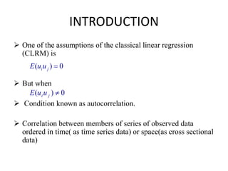
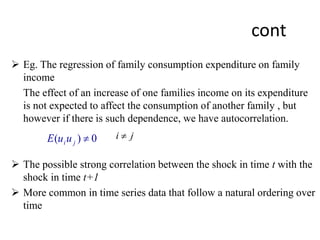
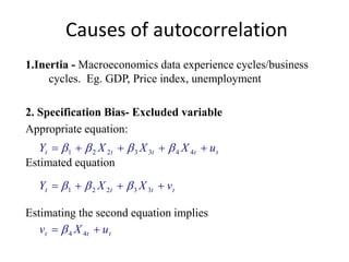
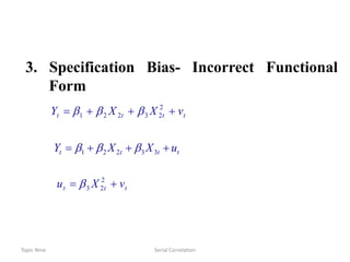
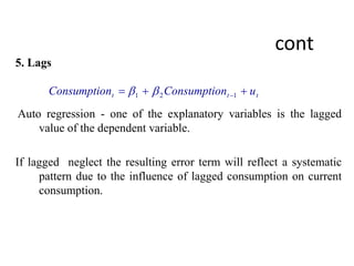
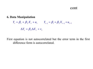
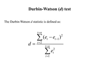
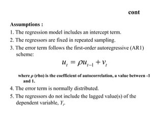
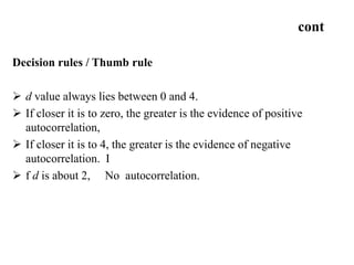
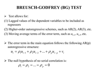
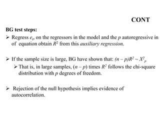
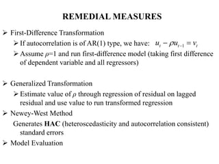
This document discusses autocorrelation, which occurs when there is a correlation between members of a series of observed data ordered over time or space. This violates an assumption of classical linear regression that error terms are uncorrelated. Causes of autocorrelation include inertia in macroeconomic data, specification bias from excluded or incorrectly specified variables, lags, data manipulation, and non-stationarity of time series data. Autocorrelation can be detected graphically or using the Durbin-Watson and Breusch-Godfrey tests. Remedial measures include first-difference transformation, generalized transformation, and using Newey-West standard errors.

1. Autocorrelation

2. INTRODUCTION
 One of the assumptions of the classical linear regression
(CLRM) is
 But when
 Condition known as autocorrelation.
 Correlation between members of series of observed data
ordered in time( as time series data) or space(as cross sectional
data)
0)( jiuuE
0)( jiuuE

3. cont
 Eg. The regression of family consumption expenditure on family
income
The effect of an increase of one families income on its expenditure
is not expected to affect the consumption of another family , but
however if there is such dependence, we have autocorrelation.
 The possible strong correlation between the shock in time t with the
shock in time t+1
 More common in time series data that follow a natural ordering over
time
ji 0)( jiuuE

4. Causes of autocorrelation
1.Inertia - Macroeconomics data experience cycles/business
cycles. Eg. GDP, Price index, unemployment
2. Specification Bias- Excluded variable
Appropriate equation:
Estimated equation
Estimating the second equation implies
ttttt uXXXY  4433221 
tttt vXXY  33221 
ttt uXv  44

5. Topic Nine Serial Correlation
3. Specification Bias- Incorrect Functional
Form
tttt vXXY  2
23221 
tttt uXXY  33221 
ttt vXu  2
23

6. cont
4. Cobweb Phenomenon
In agricultural market, the supply reacts to price with a lag of
one time period because supply decisions take time to
implement. This is known as the cobweb phenomenon.
Thus, at the beginning of this year’s planting of crops, farmers
are influenced by the price prevailing last year.

7. cont
5. Lags
Auto regression - one of the explanatory variables is the lagged
value of the dependent variable.
If lagged neglect the resulting error term will reflect a systematic
pattern due to the influence of lagged consumption on current
consumption.
ttt unConsumptionConsumptio  121 

8. cont
6. Data Manipulation
First equation is not autocorrelated but the error term in the first
difference form is autocorrelated.
ttt uXY  21  11211 
 ttt uXY 
ttt vXY  2

9. cont
7.Nonstationarity
Time series data is stationary if its characteristics (e.g. mean,
variance and covariance) are not change over time( time
variant);

10. Consequences
The OLS estimators are unbiased and consistent but inefficient
,no longer BLUE.
They are still normally distributed in large samples.
Lead R2 being unduly high.
The residual variance is likely to underestimate true varience.
In most cases standard errors are underestimated.
Thus, the hypothesis-testing procedure becomes suspect, since
the estimated standard errors may not be reliable, even in large
samples.

11. Detection of Autocorrelation
1. Graphical Method
 Can plot standardized residuals against time.
= residuals
standard error of regression
 We can also plot ut against ut-1

12. Graphical Method
Fig: No autocorrelation

13. cont
Fig: Autocorrelation

14. Durbin-Watson (d) test
The Durbin-Watson d statistic is defined as:
2
1
2
2
1
( )
t n
t t
t
t n
t
t
e e
d
e










15. cont
Assumptions :
1. The regression model includes an intercept term.
2. The regressors are fixed in repeated sampling.
3. The error term follows the first-order autoregressive (AR1)
scheme:
where ρ (rho) is the coefficient of autocorrelation, a value between -1
and 1.
4. The error term is normally distributed.
5. The regressors do not include the lagged value(s) of the
dependent variable, Yt.
1t t tu u v  

16. cont
Decision rules / Thumb rule
 d value always lies between 0 and 4.
 If closer it is to zero, the greater is the evidence of positive
autocorrelation,
 If closer it is to 4, the greater is the evidence of negative
autocorrelation. I
 f d is about 2, No autocorrelation.

17. BREUSCH-GODFREY (BG) TEST
 Test allows for:
(1) Lagged values of the dependent variables to be included as
regressors
(2) Higher-order autoregressive schemes, such as AR(2), AR(3), etc.
(3) Moving average terms of the error term, such as ut-1, ut-2, etc.
 The error term in the main equation follows the following AR(p)
autoregressive structure:
 The null hypothesis of no serial correlation is:
1 2 ... 0p     
1 1 2 2 ...t t t p t p tu u u u v        

18. CONT
BG test steps:
 Regress et, on the regressors in the model and the p autoregressive in
of equation obtain R2 from this auxiliary regression.
 If the sample size is large, BG have shown that: (n – p)R2 ~ X2
p
That is, in large samples, (n – p) times R2 follows the chi-square
distribution with p degrees of freedom.
 Rejection of the null hypothesis implies evidence of
autocorrelation.

19. REMEDIAL MEASURES
 First-Difference Transformation
If autocorrelation is of AR(1) type, we have:
Assume ρ=1 and run first-difference model (taking first difference
of dependent variable and all regressors)
 Generalized Transformation
Estimate value of ρ through regression of residual on lagged
residual and use value to run transformed regression
 Newey-West Method
Generates HAC (heteroscedasticity and autocorrelation consistent)
standard errors
 Model Evaluation
1t t tu u v  