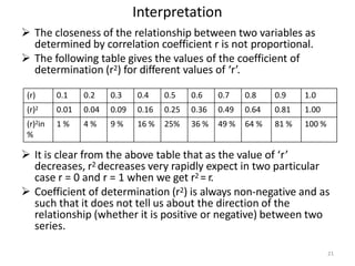
SlideShare a Scribd company logo
Correlation and Regression
1
2
Correlation
Introduction:
 Two variables are said to be correlated if the change in
one variable results in a corresponding change in the
other variable.
 The correlation is a statistical tool which studies the
relationship between two variables.
 Correlation analysis involves various methods and
techniques used for studying and measuring the extent
of the relationship between the two variables.
 Correlation is concerned with the measurement of
“strength of association between variables”.
 The degree of association between two or more
variables is termed as correlation.
3
Contd…
 Correlation analysis helps us to decide the strength of the
linear relationship between two variables.
 The word correlation is used to decide the degree of
association between variables.
 If two variables ‘x’ and ‘y’ are so related, the variables in the
magnitude of one variable tend to be accompanied by
variations in the magnitude of the other variable, they are
said to be correlated.
 Thus, correlation is a statistical tool, with the help of which,
we can determine whether or not two or more variables are
correlate and if they are correlated, what is the degree and
direction of correlation.
4
Definition
The correlation is the measure of the extent and
the direction of the relationship between two
variables in a bivariate distribution.
Example:
(i) Height and weight of children.
(ii)An increase in the price of the commodity by a
decrease in the quantity demanded.
Types of Correlation: The following are the types of
correlation
(i) Positive and Negative Correlation
(ii) Simple, Partial and Multiple Correlation
(iii) Linear and Non-linear Correlation
Contd…
Correlation first developed by Sir Francis
Galton (1822 – 1911) and then reformulated
by Karl Pearson (1857 – 1936)
Note: The degree of relationship or
association is known as the degree of
relationship.
5
6
Types of Correlation
i. Positive and Negative correlation: If both the
variables are varying in the same direction i.e. if one
variable is increasing and the other on an average is
also increasing or if as one variable is decreasing, the
other on an average, is also decreasing, correlation is
said to be positive. If on the other hand, the variable
is increasing, the other is decreasing or vice versa,
correlation is said to be negative.
Example 1: a) heights and weights (b) amount of rainfall
and yields of crops (c) price and supply of a
commodity (d) income and expenditure on luxury
goods (e) blood pressure and age
Example 2: a) price and demand of commodity (b) sales
of woolen garments and the days temperature.
7
Contd…
ii. Simple, Partial and Multiple Correlation:
When only two variables are studied, it is a
case of simple correlation. In partial and
multiple correlation, three or more variables
are studied. In multiple correlation three or
more variables are studied simultaneously. In
partial correlation, we have more than two
variables, but consider only two variables to
be influencing each other, the effect of the
other variables being kept constant.
8
Contd…
iii. Linear and Non-linear Correlation: If the
change in one variable tends to bear a
constant ratio to the change in the
other variable, the correlation is said to
be linear. Correlation is said to be non-
linear if the amount of change in one
variable does nor bear a constant ratio
to the amount of change in the other
variable.
Methods of Studying Correlation
Correlation
Graphical
Method
Scatter
Diagram
Algebraic
Method
Karl Pearson’s
Coefficient of
Correlation
9
10
Methods of Studying Correlation
 The following are the methods of determining
correlation
1. Scatter diagram method
2. Karl Pearson’s Coefficient of Correlation
1. Scatter Diagram:
 This is a graphic method of finding out relationship
between the variables.
 Given data are plotted on a graph paper in the form
of dots i.e. for each pair of x and y values we put a
dot and thus obtain as many points as the number of
observations.
 The greater the scatter of points over the graph, the
lesser the relationship between the variables.
Scatter Diagram
Perfect Positive
X
O
Y Correlation
Perfect Negative
O
Y Correlation
X
O
Low Degree of
Y Negative Correlation
Low Degree of
Positive Correlation
X
X O
Y
High Degree of
X
O
Positive Correlation
Y
O
Y
No Correlation
XO
High Degree of
Negative CorrelationY
No Correlation
X
XO
Y
11
12
Interpretation
 If all the points lie in a straight line, there is either
perfect positive or perfect negative correlation.
 If all the points lie on a straight falling from the lower
left hand corner to the upper right hand corner then the
correlation is perfect positive.
 Perfect positive if r = + 1.
 If all the points lie on a straight falling from the upper
left hand corner to the lower right hand corner then the
correlation is perfect negative.
 Perfect negative if r = -1.
 The nearer the points are to be straight line, the higher
degree of correlation.
 The farthest the points from the straight line, the lower
degree of correlation.
 If the points are widely scattered and no trend is
revealed, the variables may be un-correlated i.e. r = 0.
13
The Coefficient of Correlation:
 A scatter diagram give an idea about the type of
relationship or association between the variables
under study. It does not tell us about the
quantification of the association between the two.
 In order to quantify the relation ship between the
variables a measure called correlation coefficient
developed by Karl Pearson.
 It is defined as the measure of the degree to which
there is linear association between two intervally
scaled variables.
 Thus, the coefficient of correlation is a number which
indicates to what extent two variables are related , to
what extent variations in one go with the variations
in the other
14
Contd…
 The symbol ‘r’ or ‘rₓᵧ’ or ‘rᵧₓ’is denoted in this
method and is calculated by:
 r = {Cov(X,Y) ÷ Sₓ Sᵧ} ………..(i)
 Where Cov(X, Y) is the Sample Covariance
between X and Y.Mathematically it is defined
by
 Cov(X, Y)={∑(X–X̅)(Y–Y)}̅ ÷(n – 1)
 Sₓ = Sample standard deviation of X, is given by
 Sₓ = {∑(X – X̅)² ÷ (n – 1)}½
 Sᵧ = Sample standard deviation of Y,is givenby
 Sᵧ = {∑(Y – Y)̅² ÷ (n – 1)}½ and X̅ = ∑X ÷ n and Y̅ =
∑Y ÷ n
15
Interpretation
iii.
i. If the covariance is positive, the relationship is
positive.
ii. If the covariance is negative, the relationship is
negative.
If the covariance is zero, the variables are said to be
not correlated.
 Hence the covariance measures the strength of linear
association between considered numerical variables.
 Thus, covariance is an absolute measure of linear
association .
 In order to have relative measure of relationship it is
necessary to compute correlation coefficient .
 Computation of correlation coefficient a relation
developed by Karl Pearson are as follows:
Contd…
The formula for sample correlation coefficient (r) is calculated
by the following relation:
If (X – X̅) = x and (Y - Y̅) = y then above formula reduces to:
Example:
16
17
Properties of Karl Pearson’s Correlation Coefficient
1. The coefficient of correlation ‘r’ is always a number between -1
and +1 inclusive.
2. If r = +1 or -1, the sample points lie on a straight line.
3. If ‘r’ is near to +1 or -1, there is a strong linear association
between the variables.
4. If ‘r’ is small(close to zero), there is low degree of correlation
between the variables.
5. The coefficient of correlation is the geometric mean of the two
regression coefficients.
Symbolically: r= √(bₓᵧ . bᵧₓ)
Note: It is clear that correlation coefficient is a measure of the
degree to which the association between the two variables
approaches a linear functional relationship.
18
Interpretation of Correlation Coefficient
iii.
i. The coefficient of correlation, as obtained by the above formula shall
always lie between +1 to -1.
ii. When r = +1, there is perfect positive correlation between the
variables.
When r = -1, there is perfect negative correlation between the
variables.
iv. When r = 0, there is no correlation.
v. When r = 0.7 to 0.999, there is high degree of correlation.
vi. When r = 0.5 to 0.699, there is a moderate degree of correlation.
vii. When r is less than 0.5, there is a low degree of correlation.
viii. The value of correlation lies in between -1 to +1 i.e.
-1⩽ r ⩽ +1.
ix. The correlation coefficient is independent of the choice of both
origin and scale of observation.
x. The correlation coefficient is a pure number. It is independent of the
units of measurement.
19
Coefficient of Determination
 The coefficient of determination(r²) is the square of the
coefficient of correlation.
 It is the measure of strength of the relationship
between two variables.
 It is subject to more precise interpretation because it
can be presented as a proportion or as a percentage.
 The coefficient of determination gives the ratio of the
explained variance to the total variance.
 Thus, coefficient of determination,
r² = Explained variance ÷ Total variance
Thus, coefficient of determination shows what amount of
variability or change in independent variable is
accounted for by the variability of the dependent
variable.
20
Example
 Example 1: If r = 0.8 then r2 = (0.8)2 = 0.64 or 64%. This means that
based on the sample, 64% of the variation in dependent variable (Y), is
caused by the variations of the independent variable (X). The
remaining 36% variation in Y is unexplained by variation in X. In other
words, the variations other than X could have caused the remaining
36% variations in Y.
 Example 2: While comparing two correlation coefficients, one of which
is 0.4 and the other is 0.8 it is misleading to conclude that the
correlation in the second case is twice as high as correlation in the first
case. The coefficient of determination clearly explains this viewpoint,
since in the case r = 0.4, the coefficient of determination is r² = 0.16
and in the case r = 0.8, the coefficient of determination is r² = 0.64,
from which we conclude that correlation in the second case is four
times as high as the correlation in the first case. If the value of r = 0.8,
we cannot conclude that 80% of the variation in the relative series
(dependent variable). But the coefficient of determination in this case
is r² = 0.64 which implies that only 64% of the variation in the relative
series has been explained by the subject series and the remaining 36%
of the variation is due to other factor.
21
Interpretation
 The closeness of the relationship between two variables as
determined by correlation coefficient r is not proportional.
 The following table gives the values of the coefficient of
determination (r2) for different values of ‘r’.
 It is clear from the above table that as the value of ‘r’
decreases, r2 decreases very rapidly expect in two particular
case r = 0 and r = 1 when we get r2 = r.
 Coefficient of determination (r2) is always non-negative and as
such that it does not tell us about the direction of the
relationship (whether it is positive or negative) between two
series.
(r) 0.1 0.2 0.3 0.4 0.5 0.6 0.7 0.8 0.9 1.0
(r)2 0.01 0.04 0.09 0.16 0.25 0.36 0.49 0.64 0.81 1.00
(r)2in
%
1 % 4 % 9 % 16 % 25% 36 % 49 % 64 % 81 % 100 %
22
Test of significance of Correlation Coefficient
In order to asses whether the computed
correlation coefficient between considered
variables X and Y are statistically significant or
not t-test can be applied as test statistic. For
this the following steps can be performed:
Step 1. Formulating the Hypothesis: The
common way of starting a hypothesis is that
“The population correlation coefficient (ρ) is
zero that means there is no correlation
between X and Y variables in the population”.
Null Hypothesis, H₀: ρ = 0 ( No correlation
between X and Y variables in the population)
Contd…
Alternative Hypothesis, H₁: ρ ≠ 0 ( There is
correlation between X and Y variables in the
population) (Two tail test)
Or H₁: ρ > 0 (There is positive correlation between
X and Y variables in the population) (One tail test)
Or H₁: ρ < 0 (There is negative correlation between
X and Y variables in the population) (One tail test)
Step 2. Computing the Test Statistic: The test
statistic t for testing the existence of correlation is:
23
24
Contd…
 where; r = the sample correlation coefficient.
 ρ = the population correlation coefficient which is
hypothesized as zero.
 n= the total number of pair of observations under study.
 Step 3. Decision:
 (i) If the computed value of t is greater than table value of t
at given level of significance (α) with (n – 2) d. f. , we reject
the null hypothesis and conclude that there is evidence of
an association between considered variables.
 (ii) If the computed value of t is less than table value of t at
given level of significance (α) with (n – 2) d. f. , we accept
the null hypothesis and conclude that there is not evidence
of an association between considered variables.
 Example:
25
Simple Linear Regression
 Regression is concerned with the “Prediction” of the most
likely value of one variable when the value of the other
variable is known.
 The term regression literally means “stepping back towards
the average”.
 It was first used by British biometrician Sir Francis Galton
(1822 – 1911).
Definition: Regression analysis is a mathematical measure of
the average relationship between two or more variables in
terms of the original units of the data.
 Thus term regression is used to denote estimation or
prediction of the average value of one variable for a
specified value of the other variable.
 The estimation is done by means of suitable equation,
derived on the basis of available bivariate data. Such an
equation and its geometrical representation is called
regression curve.
26
Contd…
 In regression analysis there are two types of variables
and they are:
 i. Independent and ii. Dependent.
 Dependent variable(Y): The variable whose value is
influenced or is to be predicted is called dependent
variable.
 Independent variable(X): The variable which influences
the values or is used for prediction is called
independent variable.
 In regression analysis independent variable is known as
regressor or predictor or explanatory variable.
 In regression analysis dependent variable is known as
regressed or explained variable.
 Thus the term regression is used to denote estimation
or prediction of the average value of one variable for a
specified value of the other variable.
27
The lines of Regression
 A line fitted to a set of data points to estimates the
relationship between two variables is called regression
line.
 The regression equation of Y on X describes the
changes in the value of Y for given changes in the value
of X.
 The regression equation of X on Y describes the
changes in the value of X for given changes in the value
of Y.
 Hence, an equation for estimating a dependent variable
Y for X from the independent variable X or Y,is called
regression equation of Y on X or X on Y respectively.
 The regression equations of the regression lines, also
called least squares lines are determined by least
square method.
28
Simple Regression Model
• Simple regression line is a straight line that describe
about the dependence of the average value of one
variable on the other.
• Y = β₀ + β₁ X + Ɛ ……….(*)
• Where Y = Dependent or response or outcome variable
(Population)
• X = Independent or explanatory or predictor variable
(Population)
• β₀ = Y- intercept of the model for the population
• β₁ = population slope coefficient or population
regression coefficient. It measures the average rate of
change in dependent variable per unit change in
independent variable.
• Ɛ= Population error in Y for observation.
One unit change in x
Slope = β₁
β₀
Y- intercept
Error term
Estimated value
of y when x = x₀
Straight line
ŷ = β₀ + β₁ x
An observed value
of y when x = x₀
X
x₀ = A specific value of the
independent variable x
Y
29
Estimation of Regression Equation
Regression Model
Y = β₀ + β₁ X + Ɛ
Regression
Equation
Y = β₀ + β₁ X
Unknown
parameter
β₀ & β₁
Estimated
Regression
equation
ŷ = b₀ + b₁ x
Sample Statistics
b₀ & b₁
Sample Data:
x
x₁
x₂
.
.
xn
y
y₁
y₂
.
.
yn
b₀ & b₁
Provides estimates
of
β₀ & β₁
30
31
Model
 Linear regression model is
 Y = β₀ + β₁ X + Ɛ
 Linear regression equation is:
 Y = β₀ + β₁ X
 Sample regression model is
 ŷ= b₀ + b₁x + e
 Sample regression equation is
 ŷ= b₀ + b₁x
 Where b₀ = sample y intercept,
 b₁= sample slope coefficient
 x= independent variable
 y= dependent variable
 ŷ= estimated value of dependent variable for a given value
of independent variable.
 e = error term = y - ŷ
Least square graphically
e1
e3
e5
y2= b0+ b2x2 + e2
y1= b0+ b1x1 +e1
e4
e2
ŷi= b0+ b1xi
32
33
Least squares methods
• Let ŷ= b₀ + b₁x …..(1) be estimated linear
regression equation of y on x of the regression
equation Y = β₀ + β₁ X .
• By using the principles of least square, we can
get two normal equations of regression
equation (1) are as:
• ∑y = nb₀ +b₁ ∑x………(2)
• ∑xy = b₀∑x₁ + b₁∑x₂…….(3)
• By solving equations (2) & (3) we get the value
of b₀ & b₁ as:
Contd…
• The computational formula for y intercept b₀ as follows:
• After finding the value of b₀ & b₁, we get the required fitted
regression model of y on x as ŷ= b₀ + b₁x .
34
35
Measures of variation
• There are three measures of variations.
• They are as follows:
i. Total Sum of Squares (SST):It is a measures of
variation in the values of dependent variable (y)
around their mean value (y̅). That is
• SST = ∑(y – y)̅² = ∑y² - (∑y)²/n = ∑y² - n.y²̅ .
• Note: The total sum of squares or the total variation
is divided into the sum of two components. One is
explained variation due to the relationship between
the considered dependent variable (y) and the
independent variable (x) and the other is unexplained
variation which might be developed due to some
other factors other than the relationship between
variable x and y.
36
Contd…
ii. Regression Sum of Squares( SSR): The
regression sum of squares is the sum of the
squared differences between the predicted
value of y and the mean value of y.
• SSR = ∑(ŷ - y)̅² = b₀.∑y+b₁ ∑xy – (∑y)²/n =
b₀.∑y+b₁∑xy – n.y²
ii. Error Sum of Squares (SSE): The error sum of
square is computed as the sum of the
squared differences between the observed
value of y and the predicted value of y i.e.
• SSE = ∑(y – ŷ)² = ∑y²- b₀∑y – b₁∑xy.
Contd…
SST
SSR
y
37
X
Y
38
Contd…
Relationship: From the above figures the
relationship of SST, SSR and SSE are as follows
SST = SSR + SSE………………(i)
Where: SST = Total sum of square
SSR = Regression sum of squares
SSE = Error sum of squares
•The fit of the estimated regression line would
be best if every value of the dependent variable
y falls on the regression line.
39
Contd….
• If SSE = 0 i. e. e = (y – ŷ) = 0 then SST = SSR.
• For the perfect fit of the regression model, the
ratio of SSR to SST must be equal to unity i. e.
If SSE = 0 then the model would be perfect.
• If SSE would be larger, the fit of the regression
line would be poor.
• Note: Largest value of SSE the regression line
would be poor and if SSE = 0 the regression
line would be perfect.
40
Coefficient of Determination (r²)
• The coefficient of determination measures the
strength or extent of the association that exists
between dependent variable (y) and independent
variable (x).
• It measures the proportion of variation in the
dependent variable (y) that is explained by
independent variable of the regression line.
• Coefficient of variation measures the total
variation in the dependent variable due to the
variation in the independent variable and it is
denoted b r².
• r² = SSR/SST but SST = SSE + SSR
• then SSR = SST - SSE
• r² = 1 – (SSE/SST) = (b₀.∑y+b₁∑xy – n.y²̅ )/(∑y² – ny²̅ ).
Contd…
• Note:
i. Coefficient of determination is the square of
coefficent of correlation.
then r = ±√r²
ii. If the regression coefficient (b₁) is negative then
take the negative sign
iii. If the regression coefficient (b₁) is positive then
take the positive sign
• Adjusted coefficient of determination: The
adjusted coefficient of determination is
calculated by using the following relation:
•
41
The Standard Error of Estimates
 The standard error of estimate of Y on X, denoted by Sᵧᵪ, measures the
average variation or scatteredness of the observes data point around the
regression line. It is used to measure the reliability of the regression
equation. It is calculated by the following relation:
Interpretation of standard error of the estimate:
iii.
i. If the standard error of estimate is larger, there is greater scattering or
dispersion of the data points around the fitted line then the regression
line is poor.
ii. If the standard error is small, then there is less variation of the observed
data around the regression line. So the regression line will be better for
the predicting the dependent variable.
If the standard error is zero, it is expected that the estimating equation
would be perfect estimator of the dependent variable.
42
43
Test of Significance of Regression Coefficient in
Simple Linear Regression Model
• Totest the significance of regression
coefficient of the simple linear regression
model Y = β₀ + β₁ X + Ɛ, the following statistical
test have been applied.
i. t- test for significance in simple linear
regression.
ii. F-test for significance in simple linear
regression.
44
(i) t- test for Significance in Simple Linear Regression
• t-test is applied whether the regression
coefficient β₁ is statistically significant or not.
• The process of setting Hypothesis are as follows:
• Setting of Hypothesis:
• Null Hypothesis, H₀: β₁=0 (The population slope
(β₁) is zero between two variables X and Y in the
population.)
• Alternative Hypothesis, H₁: β₁ ≠ 0 (The population
slope (β₁) is not zero between two variables X and
Y in the population.) or H₁: β₁ > 0 or H₁: β₁ < 0
Contd…
• Test statistic: Under H₀ the test statistic is:
• Where
• This test statistic t follows t- distribution with (n – 2) d. f.
• Decisions: (i) If tcal < t tab at α % level of significance with (n-2) d.
f. then we accept H₀.
45
>t tab
• (ii) If tcal at α % level of significance with (n-2) d. f. then we
reject H₀ then we accept H₁.
46
Confidence Interval Estimating for β₁
• Another way for the linear relationship between
the variables X and Y,we can construct
confidence Interval (C. I.) estimate of β₁.
• By the help of C. I. we conclude that whether the
hypothesized value (β₁= 0) is included or not.
• For this the following formula is used:
• C. I. for β₁ = b₁ ± t(n – 2).Sb₁
• Conclusion: If this confidence interval does not
include 0(zero), then we can conclude that there
is significant relationship between the variables X
and Y.
• Example:
47
(ii) F-test for Significant in Simple Linear Regression
• F- test based on F-probability distribution can
also be applied in order to test for the
significance in regression.
• The process of setting Hypothesis are as follows:
• Setting of Hypothesis:
• Null Hypothesis, H₀: β₁=0 (The population slope
(β₁) is zero between two variables X and Y in the
population.)
• Alternative Hypothesis, H₁: β₁ ≠ 0 (The population
slope (β₁) is not zero between two variables X and
Y in the population.) or H₁: β₁ > 0 or H₁: β₁ < 0
48
Contd…
• Test statistic: F is defined as the ratio of
regression mean square (MSR) to the error mean
square (MSE).
• Where, MSR = SSR/k and MSE = SSE/(n-k-1)
• k= No. of independent variables in the regression
model. The value of k = 1 for simple linear
regression model as it has only one predictor
variable x.
• SSR = regression sum of squares = ∑(ŷ – y)̅ ²
• SSE = error sum of squares = ∑(y – ŷ)²
• The test statistic F- follows F-distribution with (n –
k – 1) i. E. (n – 2) d. f. With k = 1.
49
Contd…
• The ANOVA Table for F- statistic are summarized as:
Sources of
variation
Sum of
squares
d. f. Mean square F- ratio
Regression SSR 1 MSR = SSR/1 F = MSR / MSE
Error SSE (n – 2) MSE = SSE/n - 2
Total SST (n – 1)
• Decisions:
i. (i) If Fcal < Ftab at α % level of significance and F with 1
d. f. in the numerator and (n-2) d. f. in the
denominator then we accept H₀.
ii. (ii) If Fcal > Ftab at α % level of significance and F with1
d. f. in the numerator and (n-2) d. f. in the
denominator then we reject H₀ the accept H₁.
50
Contd…
iii. Using p- value we reject H₀ if p- value is less
than α.
• Note:
i. F- test will provide same conclusion as provided
by the t-test for only one independent variable.
ii. For simple linear regression; if t-test indicates β₁
≠ 0 and hence the F-test will also show a
significance relationship.
iii. However only the F-test can be used to test for
an overall significant relationship for the
regression with more than one independent
variable.
51
Confidence Interval Estimating of the Mean value of y.
• A point estimate is a single numerical estimate of
y is produces without any indication of ite
accuracy.
• A point estimate provides no sense of how far off
it may be from the population parameter.
• Todetermine the information a prediction or
confidence interval is developed.
• Prediction interval are used to predict particular y
values for a given value of x.
• Confidence intervals are used to estimate the
mean value of y for a given value of x.
• The point estimate of the mean value of y is same
as the point estimate of an individual value of y.
Contd…
• The formula to compute the confidence interval estimate for the mean
value of y is:
• The formula to compute the prediction interval estimate of an individual
value of y is:
• Where; ŷ = estimated or predicted value of the dependent variable
for a given value of independent variable.
• Sᵧᵪ = standard error of estimate
• t(n-2)= tabulated value of t for (n- 2) d. f. and α level of significance.
• h= hat matrix element.
• n = number of pairs of observations or sample size.
52
Interval Estimates for different values of x
X
x̅ A Given X
Y
Prediction interval for
a individual Y
Confidence interval
for the mean of Y
53

More Related Content

What's hot

Research Methodology Module-06
Research Methodology Module-06Research Methodology Module-06
Research Methodology Module-06
Kishor Ade
 
Correlation ppt...
Correlation ppt...Correlation ppt...
Correlation ppt...
Shruti Srivastava
 
Correlation and Regression Analysis using SPSS and Microsoft Excel
Correlation and Regression Analysis using SPSS and Microsoft ExcelCorrelation and Regression Analysis using SPSS and Microsoft Excel
Correlation and Regression Analysis using SPSS and Microsoft Excel
Setia Pramana
 
Linear regression and correlation analysis ppt @ bec doms
Linear regression and correlation analysis ppt @ bec domsLinear regression and correlation analysis ppt @ bec doms
Linear regression and correlation analysis ppt @ bec doms
Babasab Patil
 
Fundamental of Statistics and Types of Correlations
Fundamental of Statistics and Types of CorrelationsFundamental of Statistics and Types of Correlations
Fundamental of Statistics and Types of Correlations
Rajesh Verma
 
Correlation
CorrelationCorrelation
Correlation
James Neill
 
Chapter 16: Correlation (enhanced by VisualBee)
Chapter 16: Correlation  
(enhanced by VisualBee)Chapter 16: Correlation  
(enhanced by VisualBee)
Chapter 16: Correlation (enhanced by VisualBee)
nunngera
 
correlation and regression
correlation and regressioncorrelation and regression
correlation and regression
Keyur Tejani
 
Correlation analysis
Correlation analysisCorrelation analysis
Correlation analysis
Shivani Sharma
 
Correlation and regression
Correlation and regressionCorrelation and regression
Correlation and regression
Mohit Asija
 
Pearson Correlation, Spearman Correlation &Linear Regression
Pearson Correlation, Spearman Correlation &Linear RegressionPearson Correlation, Spearman Correlation &Linear Regression
Pearson Correlation, Spearman Correlation &Linear Regression
Azmi Mohd Tamil
 
Correlation analysis
Correlation analysis Correlation analysis
Correlation analysis
Anil Pokhrel
 
Correlation & Regression
Correlation & RegressionCorrelation & Regression
Correlation & Regression
Grant Heller
 
Correlation and regression
Correlation and regressionCorrelation and regression
Correlation and regression
Antony Raj
 
Correlation analysis
Correlation analysisCorrelation analysis
Correlation analysis
Van Martija
 
Correlation and regression
Correlation and regressionCorrelation and regression
Correlation and regression
Anil Pokhrel
 
Correlation by ramesh kumar
Correlation by ramesh kumarCorrelation by ramesh kumar
Correlation by ramesh kumar
KVS
 
Correlation
CorrelationCorrelation
Correlation
Tech_MX
 

What's hot (18)

Research Methodology Module-06
Research Methodology Module-06Research Methodology Module-06
Research Methodology Module-06
 
Correlation ppt...
Correlation ppt...Correlation ppt...
Correlation ppt...
 
Correlation and Regression Analysis using SPSS and Microsoft Excel
Correlation and Regression Analysis using SPSS and Microsoft ExcelCorrelation and Regression Analysis using SPSS and Microsoft Excel
Correlation and Regression Analysis using SPSS and Microsoft Excel
 
Linear regression and correlation analysis ppt @ bec doms
Linear regression and correlation analysis ppt @ bec domsLinear regression and correlation analysis ppt @ bec doms
Linear regression and correlation analysis ppt @ bec doms
 
Fundamental of Statistics and Types of Correlations
Fundamental of Statistics and Types of CorrelationsFundamental of Statistics and Types of Correlations
Fundamental of Statistics and Types of Correlations
 
Correlation
CorrelationCorrelation
Correlation
 
Chapter 16: Correlation (enhanced by VisualBee)
Chapter 16: Correlation  
(enhanced by VisualBee)Chapter 16: Correlation  
(enhanced by VisualBee)
Chapter 16: Correlation (enhanced by VisualBee)
 
correlation and regression
correlation and regressioncorrelation and regression
correlation and regression
 
Correlation analysis
Correlation analysisCorrelation analysis
Correlation analysis
 
Correlation and regression
Correlation and regressionCorrelation and regression
Correlation and regression
 
Pearson Correlation, Spearman Correlation &Linear Regression
Pearson Correlation, Spearman Correlation &Linear RegressionPearson Correlation, Spearman Correlation &Linear Regression
Pearson Correlation, Spearman Correlation &Linear Regression
 
Correlation analysis
Correlation analysis Correlation analysis
Correlation analysis
 
Correlation & Regression
Correlation & RegressionCorrelation & Regression
Correlation & Regression
 
Correlation and regression
Correlation and regressionCorrelation and regression
Correlation and regression
 
Correlation analysis
Correlation analysisCorrelation analysis
Correlation analysis
 
Correlation and regression
Correlation and regressionCorrelation and regression
Correlation and regression
 
Correlation by ramesh kumar
Correlation by ramesh kumarCorrelation by ramesh kumar
Correlation by ramesh kumar
 
Correlation
CorrelationCorrelation
Correlation
 

Similar to Correlation and regression impt

Correlation and Regression
Correlation and RegressionCorrelation and Regression
Correlation and Regression
Ram Kumar Shah "Struggler"
 
Study of Correlation
Study of Correlation Study of Correlation
Study of Correlation
Vikas Kumar Singh
 
PPT Correlation.pptx
PPT Correlation.pptxPPT Correlation.pptx
PPT Correlation.pptx
MahamZeeshan5
 
correlation.ppt
correlation.pptcorrelation.ppt
correlation.ppt
NayanPatil59
 
Chapter 10
Chapter 10Chapter 10
Chapter 10
guest3720ca
 
Chapter 10
Chapter 10Chapter 10
Chapter 10
Rose Jenkins
 
Correlation
CorrelationCorrelation
Correlation
Anjali Awasthi
 
Simple linear regressionn and Correlation
Simple linear regressionn and CorrelationSimple linear regressionn and Correlation
Simple linear regressionn and Correlation
Southern Range, Berhampur, Odisha
 
Simple correlation & Regression analysis
Simple correlation & Regression analysisSimple correlation & Regression analysis
Simple correlation & Regression analysis
Afra Fathima
 
2-20-04.ppt
2-20-04.ppt2-20-04.ppt
2-20-04.ppt
ayaan522797
 
Correlation Analysis for MSc in Development Finance .pdf
Correlation Analysis for MSc in Development Finance .pdfCorrelation Analysis for MSc in Development Finance .pdf
Correlation Analysis for MSc in Development Finance .pdf
ErnestNgehTingum
 
Correlation IN STATISTICS
Correlation IN STATISTICSCorrelation IN STATISTICS
Correlation IN STATISTICS
Kriace Ward
 
Correlation and regression
Correlation and regressionCorrelation and regression
Correlation and regression
Antony Raj
 
Correlation
CorrelationCorrelation
Correlation
Regent University
 
P G STAT 531 Lecture 9 Correlation
P G STAT 531 Lecture 9 CorrelationP G STAT 531 Lecture 9 Correlation
P G STAT 531 Lecture 9 Correlation
Aashish Patel
 
Correlation analysis
Correlation analysis Correlation analysis
Correlation analysis
Misab P.T
 
Correlation and Regression
Correlation and Regression Correlation and Regression
Correlation and Regression
Dr. Tushar J Bhatt
 
Correlation and Regression
Correlation and RegressionCorrelation and Regression
Correlation and Regression
Shubham Mehta
 
Correlation Analysis
Correlation AnalysisCorrelation Analysis
Correlation Analysis
Saqib Ali
 
A correlation analysis.ppt 2018
A correlation analysis.ppt 2018A correlation analysis.ppt 2018
A correlation analysis.ppt 2018
DrRavindraKumarSaini
 

Similar to Correlation and regression impt (20)

Correlation and Regression
Correlation and RegressionCorrelation and Regression
Correlation and Regression
 
Study of Correlation
Study of Correlation Study of Correlation
Study of Correlation
 
PPT Correlation.pptx
PPT Correlation.pptxPPT Correlation.pptx
PPT Correlation.pptx
 
correlation.ppt
correlation.pptcorrelation.ppt
correlation.ppt
 
Chapter 10
Chapter 10Chapter 10
Chapter 10
 
Chapter 10
Chapter 10Chapter 10
Chapter 10
 
Correlation
CorrelationCorrelation
Correlation
 
Simple linear regressionn and Correlation
Simple linear regressionn and CorrelationSimple linear regressionn and Correlation
Simple linear regressionn and Correlation
 
Simple correlation & Regression analysis
Simple correlation & Regression analysisSimple correlation & Regression analysis
Simple correlation & Regression analysis
 
2-20-04.ppt
2-20-04.ppt2-20-04.ppt
2-20-04.ppt
 
Correlation Analysis for MSc in Development Finance .pdf
Correlation Analysis for MSc in Development Finance .pdfCorrelation Analysis for MSc in Development Finance .pdf
Correlation Analysis for MSc in Development Finance .pdf
 
Correlation IN STATISTICS
Correlation IN STATISTICSCorrelation IN STATISTICS
Correlation IN STATISTICS
 
Correlation and regression
Correlation and regressionCorrelation and regression
Correlation and regression
 
Correlation
CorrelationCorrelation
Correlation
 
P G STAT 531 Lecture 9 Correlation
P G STAT 531 Lecture 9 CorrelationP G STAT 531 Lecture 9 Correlation
P G STAT 531 Lecture 9 Correlation
 
Correlation analysis
Correlation analysis Correlation analysis
Correlation analysis
 
Correlation and Regression
Correlation and Regression Correlation and Regression
Correlation and Regression
 
Correlation and Regression
Correlation and RegressionCorrelation and Regression
Correlation and Regression
 
Correlation Analysis
Correlation AnalysisCorrelation Analysis
Correlation Analysis
 
A correlation analysis.ppt 2018
A correlation analysis.ppt 2018A correlation analysis.ppt 2018
A correlation analysis.ppt 2018
 

More from freelancer

PPT1KM.pptx
PPT1KM.pptxPPT1KM.pptx
PPT1KM.pptx
freelancer
 
KNOWLEDGE MANAGEMENT notes.docx
KNOWLEDGE MANAGEMENT notes.docxKNOWLEDGE MANAGEMENT notes.docx
KNOWLEDGE MANAGEMENT notes.docx
freelancer
 
KNOWLEDGE MANAGEMENT notes.docx
KNOWLEDGE MANAGEMENT notes.docxKNOWLEDGE MANAGEMENT notes.docx
KNOWLEDGE MANAGEMENT notes.docx
freelancer
 
academic model.docx
academic model.docxacademic model.docx
academic model.docx
freelancer
 
AI BASICS.ppt
AI BASICS.pptAI BASICS.ppt
AI BASICS.ppt
freelancer
 
Three Statement Model.pptx
Three Statement Model.pptxThree Statement Model.pptx
Three Statement Model.pptx
freelancer
 
Conjoint Analysis.pptx
Conjoint Analysis.pptxConjoint Analysis.pptx
Conjoint Analysis.pptx
freelancer
 
Conjoint analysis
Conjoint analysisConjoint analysis
Conjoint analysis
freelancer
 
Demography ppt2
Demography ppt2Demography ppt2
Demography ppt2
freelancer
 
Chapter 4-analytics-talent-management
Chapter 4-analytics-talent-managementChapter 4-analytics-talent-management
Chapter 4-analytics-talent-management
freelancer
 
Tabulation
TabulationTabulation
Tabulation
freelancer
 
The t test
The t testThe t test
The t test
freelancer
 

More from freelancer (12)

PPT1KM.pptx
PPT1KM.pptxPPT1KM.pptx
PPT1KM.pptx
 
KNOWLEDGE MANAGEMENT notes.docx
KNOWLEDGE MANAGEMENT notes.docxKNOWLEDGE MANAGEMENT notes.docx
KNOWLEDGE MANAGEMENT notes.docx
 
KNOWLEDGE MANAGEMENT notes.docx
KNOWLEDGE MANAGEMENT notes.docxKNOWLEDGE MANAGEMENT notes.docx
KNOWLEDGE MANAGEMENT notes.docx
 
academic model.docx
academic model.docxacademic model.docx
academic model.docx
 
AI BASICS.ppt
AI BASICS.pptAI BASICS.ppt
AI BASICS.ppt
 
Three Statement Model.pptx
Three Statement Model.pptxThree Statement Model.pptx
Three Statement Model.pptx
 
Conjoint Analysis.pptx
Conjoint Analysis.pptxConjoint Analysis.pptx
Conjoint Analysis.pptx
 
Conjoint analysis
Conjoint analysisConjoint analysis
Conjoint analysis
 
Demography ppt2
Demography ppt2Demography ppt2
Demography ppt2
 
Chapter 4-analytics-talent-management
Chapter 4-analytics-talent-managementChapter 4-analytics-talent-management
Chapter 4-analytics-talent-management
 
Tabulation
TabulationTabulation
Tabulation
 
The t test
The t testThe t test
The t test
 

Recently uploaded

Chapter 12 - climate change and the energy crisis
Chapter 12 - climate change and the energy crisisChapter 12 - climate change and the energy crisis
Chapter 12 - climate change and the energy crisis
tonzsalvador2222
 
The use of Nauplii and metanauplii artemia in aquaculture (brine shrimp).pptx
The use of Nauplii and metanauplii artemia in aquaculture (brine shrimp).pptxThe use of Nauplii and metanauplii artemia in aquaculture (brine shrimp).pptx
The use of Nauplii and metanauplii artemia in aquaculture (brine shrimp).pptx
MAGOTI ERNEST
 
Micronuclei test.M.sc.zoology.fisheries.
Micronuclei test.M.sc.zoology.fisheries.Micronuclei test.M.sc.zoology.fisheries.
Micronuclei test.M.sc.zoology.fisheries.
Aditi Bajpai
 
Unlocking the mysteries of reproduction: Exploring fecundity and gonadosomati...
Unlocking the mysteries of reproduction: Exploring fecundity and gonadosomati...Unlocking the mysteries of reproduction: Exploring fecundity and gonadosomati...
Unlocking the mysteries of reproduction: Exploring fecundity and gonadosomati...
AbdullaAlAsif1
 
NuGOweek 2024 Ghent programme overview flyer
NuGOweek 2024 Ghent programme overview flyerNuGOweek 2024 Ghent programme overview flyer
NuGOweek 2024 Ghent programme overview flyer
pablovgd
 
Eukaryotic Transcription Presentation.pptx
Eukaryotic Transcription Presentation.pptxEukaryotic Transcription Presentation.pptx
Eukaryotic Transcription Presentation.pptx
RitabrataSarkar3
 
Sharlene Leurig - Enabling Onsite Water Use with Net Zero Water
Sharlene Leurig - Enabling Onsite Water Use with Net Zero WaterSharlene Leurig - Enabling Onsite Water Use with Net Zero Water
Sharlene Leurig - Enabling Onsite Water Use with Net Zero Water
Texas Alliance of Groundwater Districts
 
mô tả các thí nghiệm về đánh giá tác động dòng khí hóa sau đốt
mô tả các thí nghiệm về đánh giá tác động dòng khí hóa sau đốtmô tả các thí nghiệm về đánh giá tác động dòng khí hóa sau đốt
mô tả các thí nghiệm về đánh giá tác động dòng khí hóa sau đốt
HongcNguyn6
 
Phenomics assisted breeding in crop improvement
Phenomics assisted breeding in crop improvementPhenomics assisted breeding in crop improvement
Phenomics assisted breeding in crop improvement
IshaGoswami9
 
ESR spectroscopy in liquid food and beverages.pptx
ESR spectroscopy in liquid food and beverages.pptxESR spectroscopy in liquid food and beverages.pptx
ESR spectroscopy in liquid food and beverages.pptx
PRIYANKA PATEL
 
Deep Software Variability and Frictionless Reproducibility
Deep Software Variability and Frictionless ReproducibilityDeep Software Variability and Frictionless Reproducibility
Deep Software Variability and Frictionless Reproducibility
University of Rennes, INSA Rennes, Inria/IRISA, CNRS
 
molar-distalization in orthodontics-seminar.pptx
molar-distalization in orthodontics-seminar.pptxmolar-distalization in orthodontics-seminar.pptx
molar-distalization in orthodontics-seminar.pptx
Anagha Prasad
 
The binding of cosmological structures by massless topological defects
The binding of cosmological structures by massless topological defectsThe binding of cosmological structures by massless topological defects
The binding of cosmological structures by massless topological defects
Sérgio Sacani
 
Topic: SICKLE CELL DISEASE IN CHILDREN-3.pdf
Topic: SICKLE CELL DISEASE IN CHILDREN-3.pdfTopic: SICKLE CELL DISEASE IN CHILDREN-3.pdf
Topic: SICKLE CELL DISEASE IN CHILDREN-3.pdf
TinyAnderson
 
Cytokines and their role in immune regulation.pptx
Cytokines and their role in immune regulation.pptxCytokines and their role in immune regulation.pptx
Cytokines and their role in immune regulation.pptx
Hitesh Sikarwar
 
3D Hybrid PIC simulation of the plasma expansion (ISSS-14)
3D Hybrid PIC simulation of the plasma expansion (ISSS-14)3D Hybrid PIC simulation of the plasma expansion (ISSS-14)
3D Hybrid PIC simulation of the plasma expansion (ISSS-14)
David Osipyan
 
Nucleophilic Addition of carbonyl compounds.pptx
Nucleophilic Addition of carbonyl  compounds.pptxNucleophilic Addition of carbonyl  compounds.pptx
Nucleophilic Addition of carbonyl compounds.pptx
SSR02
 
Bob Reedy - Nitrate in Texas Groundwater.pdf
Bob Reedy - Nitrate in Texas Groundwater.pdfBob Reedy - Nitrate in Texas Groundwater.pdf
Bob Reedy - Nitrate in Texas Groundwater.pdf
Texas Alliance of Groundwater Districts
 
Remote Sensing and Computational, Evolutionary, Supercomputing, and Intellige...
Remote Sensing and Computational, Evolutionary, Supercomputing, and Intellige...Remote Sensing and Computational, Evolutionary, Supercomputing, and Intellige...
Remote Sensing and Computational, Evolutionary, Supercomputing, and Intellige...
University of Maribor
 
原版制作(carleton毕业证书)卡尔顿大学毕业证硕士文凭原版一模一样
原版制作(carleton毕业证书)卡尔顿大学毕业证硕士文凭原版一模一样原版制作(carleton毕业证书)卡尔顿大学毕业证硕士文凭原版一模一样
原版制作(carleton毕业证书)卡尔顿大学毕业证硕士文凭原版一模一样
yqqaatn0
 

Recently uploaded (20)

Chapter 12 - climate change and the energy crisis
Chapter 12 - climate change and the energy crisisChapter 12 - climate change and the energy crisis
Chapter 12 - climate change and the energy crisis
 
The use of Nauplii and metanauplii artemia in aquaculture (brine shrimp).pptx
The use of Nauplii and metanauplii artemia in aquaculture (brine shrimp).pptxThe use of Nauplii and metanauplii artemia in aquaculture (brine shrimp).pptx
The use of Nauplii and metanauplii artemia in aquaculture (brine shrimp).pptx
 
Micronuclei test.M.sc.zoology.fisheries.
Micronuclei test.M.sc.zoology.fisheries.Micronuclei test.M.sc.zoology.fisheries.
Micronuclei test.M.sc.zoology.fisheries.
 
Unlocking the mysteries of reproduction: Exploring fecundity and gonadosomati...
Unlocking the mysteries of reproduction: Exploring fecundity and gonadosomati...Unlocking the mysteries of reproduction: Exploring fecundity and gonadosomati...
Unlocking the mysteries of reproduction: Exploring fecundity and gonadosomati...
 
NuGOweek 2024 Ghent programme overview flyer
NuGOweek 2024 Ghent programme overview flyerNuGOweek 2024 Ghent programme overview flyer
NuGOweek 2024 Ghent programme overview flyer
 
Eukaryotic Transcription Presentation.pptx
Eukaryotic Transcription Presentation.pptxEukaryotic Transcription Presentation.pptx
Eukaryotic Transcription Presentation.pptx
 
Sharlene Leurig - Enabling Onsite Water Use with Net Zero Water
Sharlene Leurig - Enabling Onsite Water Use with Net Zero WaterSharlene Leurig - Enabling Onsite Water Use with Net Zero Water
Sharlene Leurig - Enabling Onsite Water Use with Net Zero Water
 
mô tả các thí nghiệm về đánh giá tác động dòng khí hóa sau đốt
mô tả các thí nghiệm về đánh giá tác động dòng khí hóa sau đốtmô tả các thí nghiệm về đánh giá tác động dòng khí hóa sau đốt
mô tả các thí nghiệm về đánh giá tác động dòng khí hóa sau đốt
 
Phenomics assisted breeding in crop improvement
Phenomics assisted breeding in crop improvementPhenomics assisted breeding in crop improvement
Phenomics assisted breeding in crop improvement
 
ESR spectroscopy in liquid food and beverages.pptx
ESR spectroscopy in liquid food and beverages.pptxESR spectroscopy in liquid food and beverages.pptx
ESR spectroscopy in liquid food and beverages.pptx
 
Deep Software Variability and Frictionless Reproducibility
Deep Software Variability and Frictionless ReproducibilityDeep Software Variability and Frictionless Reproducibility
Deep Software Variability and Frictionless Reproducibility
 
molar-distalization in orthodontics-seminar.pptx
molar-distalization in orthodontics-seminar.pptxmolar-distalization in orthodontics-seminar.pptx
molar-distalization in orthodontics-seminar.pptx
 
The binding of cosmological structures by massless topological defects
The binding of cosmological structures by massless topological defectsThe binding of cosmological structures by massless topological defects
The binding of cosmological structures by massless topological defects
 
Topic: SICKLE CELL DISEASE IN CHILDREN-3.pdf
Topic: SICKLE CELL DISEASE IN CHILDREN-3.pdfTopic: SICKLE CELL DISEASE IN CHILDREN-3.pdf
Topic: SICKLE CELL DISEASE IN CHILDREN-3.pdf
 
Cytokines and their role in immune regulation.pptx
Cytokines and their role in immune regulation.pptxCytokines and their role in immune regulation.pptx
Cytokines and their role in immune regulation.pptx
 
3D Hybrid PIC simulation of the plasma expansion (ISSS-14)
3D Hybrid PIC simulation of the plasma expansion (ISSS-14)3D Hybrid PIC simulation of the plasma expansion (ISSS-14)
3D Hybrid PIC simulation of the plasma expansion (ISSS-14)
 
Nucleophilic Addition of carbonyl compounds.pptx
Nucleophilic Addition of carbonyl  compounds.pptxNucleophilic Addition of carbonyl  compounds.pptx
Nucleophilic Addition of carbonyl compounds.pptx
 
Bob Reedy - Nitrate in Texas Groundwater.pdf
Bob Reedy - Nitrate in Texas Groundwater.pdfBob Reedy - Nitrate in Texas Groundwater.pdf
Bob Reedy - Nitrate in Texas Groundwater.pdf
 
Remote Sensing and Computational, Evolutionary, Supercomputing, and Intellige...
Remote Sensing and Computational, Evolutionary, Supercomputing, and Intellige...Remote Sensing and Computational, Evolutionary, Supercomputing, and Intellige...
Remote Sensing and Computational, Evolutionary, Supercomputing, and Intellige...
 
原版制作(carleton毕业证书)卡尔顿大学毕业证硕士文凭原版一模一样
原版制作(carleton毕业证书)卡尔顿大学毕业证硕士文凭原版一模一样原版制作(carleton毕业证书)卡尔顿大学毕业证硕士文凭原版一模一样
原版制作(carleton毕业证书)卡尔顿大学毕业证硕士文凭原版一模一样
 

Correlation and regression impt

  • 2. 2 Correlation Introduction:  Two variables are said to be correlated if the change in one variable results in a corresponding change in the other variable.  The correlation is a statistical tool which studies the relationship between two variables.  Correlation analysis involves various methods and techniques used for studying and measuring the extent of the relationship between the two variables.  Correlation is concerned with the measurement of “strength of association between variables”.  The degree of association between two or more variables is termed as correlation.
  • 3. 3 Contd…  Correlation analysis helps us to decide the strength of the linear relationship between two variables.  The word correlation is used to decide the degree of association between variables.  If two variables ‘x’ and ‘y’ are so related, the variables in the magnitude of one variable tend to be accompanied by variations in the magnitude of the other variable, they are said to be correlated.  Thus, correlation is a statistical tool, with the help of which, we can determine whether or not two or more variables are correlate and if they are correlated, what is the degree and direction of correlation.
  • 4. 4 Definition The correlation is the measure of the extent and the direction of the relationship between two variables in a bivariate distribution. Example: (i) Height and weight of children. (ii)An increase in the price of the commodity by a decrease in the quantity demanded. Types of Correlation: The following are the types of correlation (i) Positive and Negative Correlation (ii) Simple, Partial and Multiple Correlation (iii) Linear and Non-linear Correlation
  • 5. Contd… Correlation first developed by Sir Francis Galton (1822 – 1911) and then reformulated by Karl Pearson (1857 – 1936) Note: The degree of relationship or association is known as the degree of relationship. 5
  • 6. 6 Types of Correlation i. Positive and Negative correlation: If both the variables are varying in the same direction i.e. if one variable is increasing and the other on an average is also increasing or if as one variable is decreasing, the other on an average, is also decreasing, correlation is said to be positive. If on the other hand, the variable is increasing, the other is decreasing or vice versa, correlation is said to be negative. Example 1: a) heights and weights (b) amount of rainfall and yields of crops (c) price and supply of a commodity (d) income and expenditure on luxury goods (e) blood pressure and age Example 2: a) price and demand of commodity (b) sales of woolen garments and the days temperature.
  • 7. 7 Contd… ii. Simple, Partial and Multiple Correlation: When only two variables are studied, it is a case of simple correlation. In partial and multiple correlation, three or more variables are studied. In multiple correlation three or more variables are studied simultaneously. In partial correlation, we have more than two variables, but consider only two variables to be influencing each other, the effect of the other variables being kept constant.
  • 8. 8 Contd… iii. Linear and Non-linear Correlation: If the change in one variable tends to bear a constant ratio to the change in the other variable, the correlation is said to be linear. Correlation is said to be non- linear if the amount of change in one variable does nor bear a constant ratio to the amount of change in the other variable.
  • 9. Methods of Studying Correlation Correlation Graphical Method Scatter Diagram Algebraic Method Karl Pearson’s Coefficient of Correlation 9
  • 10. 10 Methods of Studying Correlation  The following are the methods of determining correlation 1. Scatter diagram method 2. Karl Pearson’s Coefficient of Correlation 1. Scatter Diagram:  This is a graphic method of finding out relationship between the variables.  Given data are plotted on a graph paper in the form of dots i.e. for each pair of x and y values we put a dot and thus obtain as many points as the number of observations.  The greater the scatter of points over the graph, the lesser the relationship between the variables.
  • 11. Scatter Diagram Perfect Positive X O Y Correlation Perfect Negative O Y Correlation X O Low Degree of Y Negative Correlation Low Degree of Positive Correlation X X O Y High Degree of X O Positive Correlation Y O Y No Correlation XO High Degree of Negative CorrelationY No Correlation X XO Y 11
  • 12. 12 Interpretation  If all the points lie in a straight line, there is either perfect positive or perfect negative correlation.  If all the points lie on a straight falling from the lower left hand corner to the upper right hand corner then the correlation is perfect positive.  Perfect positive if r = + 1.  If all the points lie on a straight falling from the upper left hand corner to the lower right hand corner then the correlation is perfect negative.  Perfect negative if r = -1.  The nearer the points are to be straight line, the higher degree of correlation.  The farthest the points from the straight line, the lower degree of correlation.  If the points are widely scattered and no trend is revealed, the variables may be un-correlated i.e. r = 0.
  • 13. 13 The Coefficient of Correlation:  A scatter diagram give an idea about the type of relationship or association between the variables under study. It does not tell us about the quantification of the association between the two.  In order to quantify the relation ship between the variables a measure called correlation coefficient developed by Karl Pearson.  It is defined as the measure of the degree to which there is linear association between two intervally scaled variables.  Thus, the coefficient of correlation is a number which indicates to what extent two variables are related , to what extent variations in one go with the variations in the other
  • 14. 14 Contd…  The symbol ‘r’ or ‘rₓᵧ’ or ‘rᵧₓ’is denoted in this method and is calculated by:  r = {Cov(X,Y) ÷ Sₓ Sᵧ} ………..(i)  Where Cov(X, Y) is the Sample Covariance between X and Y.Mathematically it is defined by  Cov(X, Y)={∑(X–X̅)(Y–Y)}̅ ÷(n – 1)  Sₓ = Sample standard deviation of X, is given by  Sₓ = {∑(X – X̅)² ÷ (n – 1)}½  Sᵧ = Sample standard deviation of Y,is givenby  Sᵧ = {∑(Y – Y)̅² ÷ (n – 1)}½ and X̅ = ∑X ÷ n and Y̅ = ∑Y ÷ n
  • 15. 15 Interpretation iii. i. If the covariance is positive, the relationship is positive. ii. If the covariance is negative, the relationship is negative. If the covariance is zero, the variables are said to be not correlated.  Hence the covariance measures the strength of linear association between considered numerical variables.  Thus, covariance is an absolute measure of linear association .  In order to have relative measure of relationship it is necessary to compute correlation coefficient .  Computation of correlation coefficient a relation developed by Karl Pearson are as follows:
  • 16. Contd… The formula for sample correlation coefficient (r) is calculated by the following relation: If (X – X̅) = x and (Y - Y̅) = y then above formula reduces to: Example: 16
  • 17. 17 Properties of Karl Pearson’s Correlation Coefficient 1. The coefficient of correlation ‘r’ is always a number between -1 and +1 inclusive. 2. If r = +1 or -1, the sample points lie on a straight line. 3. If ‘r’ is near to +1 or -1, there is a strong linear association between the variables. 4. If ‘r’ is small(close to zero), there is low degree of correlation between the variables. 5. The coefficient of correlation is the geometric mean of the two regression coefficients. Symbolically: r= √(bₓᵧ . bᵧₓ) Note: It is clear that correlation coefficient is a measure of the degree to which the association between the two variables approaches a linear functional relationship.
  • 18. 18 Interpretation of Correlation Coefficient iii. i. The coefficient of correlation, as obtained by the above formula shall always lie between +1 to -1. ii. When r = +1, there is perfect positive correlation between the variables. When r = -1, there is perfect negative correlation between the variables. iv. When r = 0, there is no correlation. v. When r = 0.7 to 0.999, there is high degree of correlation. vi. When r = 0.5 to 0.699, there is a moderate degree of correlation. vii. When r is less than 0.5, there is a low degree of correlation. viii. The value of correlation lies in between -1 to +1 i.e. -1⩽ r ⩽ +1. ix. The correlation coefficient is independent of the choice of both origin and scale of observation. x. The correlation coefficient is a pure number. It is independent of the units of measurement.
  • 19. 19 Coefficient of Determination  The coefficient of determination(r²) is the square of the coefficient of correlation.  It is the measure of strength of the relationship between two variables.  It is subject to more precise interpretation because it can be presented as a proportion or as a percentage.  The coefficient of determination gives the ratio of the explained variance to the total variance.  Thus, coefficient of determination, r² = Explained variance ÷ Total variance Thus, coefficient of determination shows what amount of variability or change in independent variable is accounted for by the variability of the dependent variable.
  • 20. 20 Example  Example 1: If r = 0.8 then r2 = (0.8)2 = 0.64 or 64%. This means that based on the sample, 64% of the variation in dependent variable (Y), is caused by the variations of the independent variable (X). The remaining 36% variation in Y is unexplained by variation in X. In other words, the variations other than X could have caused the remaining 36% variations in Y.  Example 2: While comparing two correlation coefficients, one of which is 0.4 and the other is 0.8 it is misleading to conclude that the correlation in the second case is twice as high as correlation in the first case. The coefficient of determination clearly explains this viewpoint, since in the case r = 0.4, the coefficient of determination is r² = 0.16 and in the case r = 0.8, the coefficient of determination is r² = 0.64, from which we conclude that correlation in the second case is four times as high as the correlation in the first case. If the value of r = 0.8, we cannot conclude that 80% of the variation in the relative series (dependent variable). But the coefficient of determination in this case is r² = 0.64 which implies that only 64% of the variation in the relative series has been explained by the subject series and the remaining 36% of the variation is due to other factor.
  • 21. 21 Interpretation  The closeness of the relationship between two variables as determined by correlation coefficient r is not proportional.  The following table gives the values of the coefficient of determination (r2) for different values of ‘r’.  It is clear from the above table that as the value of ‘r’ decreases, r2 decreases very rapidly expect in two particular case r = 0 and r = 1 when we get r2 = r.  Coefficient of determination (r2) is always non-negative and as such that it does not tell us about the direction of the relationship (whether it is positive or negative) between two series. (r) 0.1 0.2 0.3 0.4 0.5 0.6 0.7 0.8 0.9 1.0 (r)2 0.01 0.04 0.09 0.16 0.25 0.36 0.49 0.64 0.81 1.00 (r)2in % 1 % 4 % 9 % 16 % 25% 36 % 49 % 64 % 81 % 100 %
  • 22. 22 Test of significance of Correlation Coefficient In order to asses whether the computed correlation coefficient between considered variables X and Y are statistically significant or not t-test can be applied as test statistic. For this the following steps can be performed: Step 1. Formulating the Hypothesis: The common way of starting a hypothesis is that “The population correlation coefficient (ρ) is zero that means there is no correlation between X and Y variables in the population”. Null Hypothesis, H₀: ρ = 0 ( No correlation between X and Y variables in the population)
  • 23. Contd… Alternative Hypothesis, H₁: ρ ≠ 0 ( There is correlation between X and Y variables in the population) (Two tail test) Or H₁: ρ > 0 (There is positive correlation between X and Y variables in the population) (One tail test) Or H₁: ρ < 0 (There is negative correlation between X and Y variables in the population) (One tail test) Step 2. Computing the Test Statistic: The test statistic t for testing the existence of correlation is: 23
  • 24. 24 Contd…  where; r = the sample correlation coefficient.  ρ = the population correlation coefficient which is hypothesized as zero.  n= the total number of pair of observations under study.  Step 3. Decision:  (i) If the computed value of t is greater than table value of t at given level of significance (α) with (n – 2) d. f. , we reject the null hypothesis and conclude that there is evidence of an association between considered variables.  (ii) If the computed value of t is less than table value of t at given level of significance (α) with (n – 2) d. f. , we accept the null hypothesis and conclude that there is not evidence of an association between considered variables.  Example:
  • 25. 25 Simple Linear Regression  Regression is concerned with the “Prediction” of the most likely value of one variable when the value of the other variable is known.  The term regression literally means “stepping back towards the average”.  It was first used by British biometrician Sir Francis Galton (1822 – 1911). Definition: Regression analysis is a mathematical measure of the average relationship between two or more variables in terms of the original units of the data.  Thus term regression is used to denote estimation or prediction of the average value of one variable for a specified value of the other variable.  The estimation is done by means of suitable equation, derived on the basis of available bivariate data. Such an equation and its geometrical representation is called regression curve.
  • 26. 26 Contd…  In regression analysis there are two types of variables and they are:  i. Independent and ii. Dependent.  Dependent variable(Y): The variable whose value is influenced or is to be predicted is called dependent variable.  Independent variable(X): The variable which influences the values or is used for prediction is called independent variable.  In regression analysis independent variable is known as regressor or predictor or explanatory variable.  In regression analysis dependent variable is known as regressed or explained variable.  Thus the term regression is used to denote estimation or prediction of the average value of one variable for a specified value of the other variable.
  • 27. 27 The lines of Regression  A line fitted to a set of data points to estimates the relationship between two variables is called regression line.  The regression equation of Y on X describes the changes in the value of Y for given changes in the value of X.  The regression equation of X on Y describes the changes in the value of X for given changes in the value of Y.  Hence, an equation for estimating a dependent variable Y for X from the independent variable X or Y,is called regression equation of Y on X or X on Y respectively.  The regression equations of the regression lines, also called least squares lines are determined by least square method.
  • 28. 28 Simple Regression Model • Simple regression line is a straight line that describe about the dependence of the average value of one variable on the other. • Y = β₀ + β₁ X + Ɛ ……….(*) • Where Y = Dependent or response or outcome variable (Population) • X = Independent or explanatory or predictor variable (Population) • β₀ = Y- intercept of the model for the population • β₁ = population slope coefficient or population regression coefficient. It measures the average rate of change in dependent variable per unit change in independent variable. • Ɛ= Population error in Y for observation.
  • 29. One unit change in x Slope = β₁ β₀ Y- intercept Error term Estimated value of y when x = x₀ Straight line ŷ = β₀ + β₁ x An observed value of y when x = x₀ X x₀ = A specific value of the independent variable x Y 29
  • 30. Estimation of Regression Equation Regression Model Y = β₀ + β₁ X + Ɛ Regression Equation Y = β₀ + β₁ X Unknown parameter β₀ & β₁ Estimated Regression equation ŷ = b₀ + b₁ x Sample Statistics b₀ & b₁ Sample Data: x x₁ x₂ . . xn y y₁ y₂ . . yn b₀ & b₁ Provides estimates of β₀ & β₁ 30
  • 31. 31 Model  Linear regression model is  Y = β₀ + β₁ X + Ɛ  Linear regression equation is:  Y = β₀ + β₁ X  Sample regression model is  ŷ= b₀ + b₁x + e  Sample regression equation is  ŷ= b₀ + b₁x  Where b₀ = sample y intercept,  b₁= sample slope coefficient  x= independent variable  y= dependent variable  ŷ= estimated value of dependent variable for a given value of independent variable.  e = error term = y - ŷ
  • 32. Least square graphically e1 e3 e5 y2= b0+ b2x2 + e2 y1= b0+ b1x1 +e1 e4 e2 ŷi= b0+ b1xi 32
  • 33. 33 Least squares methods • Let ŷ= b₀ + b₁x …..(1) be estimated linear regression equation of y on x of the regression equation Y = β₀ + β₁ X . • By using the principles of least square, we can get two normal equations of regression equation (1) are as: • ∑y = nb₀ +b₁ ∑x………(2) • ∑xy = b₀∑x₁ + b₁∑x₂…….(3) • By solving equations (2) & (3) we get the value of b₀ & b₁ as:
  • 34. Contd… • The computational formula for y intercept b₀ as follows: • After finding the value of b₀ & b₁, we get the required fitted regression model of y on x as ŷ= b₀ + b₁x . 34
  • 35. 35 Measures of variation • There are three measures of variations. • They are as follows: i. Total Sum of Squares (SST):It is a measures of variation in the values of dependent variable (y) around their mean value (y̅). That is • SST = ∑(y – y)̅² = ∑y² - (∑y)²/n = ∑y² - n.y²̅ . • Note: The total sum of squares or the total variation is divided into the sum of two components. One is explained variation due to the relationship between the considered dependent variable (y) and the independent variable (x) and the other is unexplained variation which might be developed due to some other factors other than the relationship between variable x and y.
  • 36. 36 Contd… ii. Regression Sum of Squares( SSR): The regression sum of squares is the sum of the squared differences between the predicted value of y and the mean value of y. • SSR = ∑(ŷ - y)̅² = b₀.∑y+b₁ ∑xy – (∑y)²/n = b₀.∑y+b₁∑xy – n.y² ii. Error Sum of Squares (SSE): The error sum of square is computed as the sum of the squared differences between the observed value of y and the predicted value of y i.e. • SSE = ∑(y – ŷ)² = ∑y²- b₀∑y – b₁∑xy.
  • 38. 38 Contd… Relationship: From the above figures the relationship of SST, SSR and SSE are as follows SST = SSR + SSE………………(i) Where: SST = Total sum of square SSR = Regression sum of squares SSE = Error sum of squares •The fit of the estimated regression line would be best if every value of the dependent variable y falls on the regression line.
  • 39. 39 Contd…. • If SSE = 0 i. e. e = (y – ŷ) = 0 then SST = SSR. • For the perfect fit of the regression model, the ratio of SSR to SST must be equal to unity i. e. If SSE = 0 then the model would be perfect. • If SSE would be larger, the fit of the regression line would be poor. • Note: Largest value of SSE the regression line would be poor and if SSE = 0 the regression line would be perfect.
  • 40. 40 Coefficient of Determination (r²) • The coefficient of determination measures the strength or extent of the association that exists between dependent variable (y) and independent variable (x). • It measures the proportion of variation in the dependent variable (y) that is explained by independent variable of the regression line. • Coefficient of variation measures the total variation in the dependent variable due to the variation in the independent variable and it is denoted b r². • r² = SSR/SST but SST = SSE + SSR • then SSR = SST - SSE • r² = 1 – (SSE/SST) = (b₀.∑y+b₁∑xy – n.y²̅ )/(∑y² – ny²̅ ).
  • 41. Contd… • Note: i. Coefficient of determination is the square of coefficent of correlation. then r = ±√r² ii. If the regression coefficient (b₁) is negative then take the negative sign iii. If the regression coefficient (b₁) is positive then take the positive sign • Adjusted coefficient of determination: The adjusted coefficient of determination is calculated by using the following relation: • 41
  • 42. The Standard Error of Estimates  The standard error of estimate of Y on X, denoted by Sᵧᵪ, measures the average variation or scatteredness of the observes data point around the regression line. It is used to measure the reliability of the regression equation. It is calculated by the following relation: Interpretation of standard error of the estimate: iii. i. If the standard error of estimate is larger, there is greater scattering or dispersion of the data points around the fitted line then the regression line is poor. ii. If the standard error is small, then there is less variation of the observed data around the regression line. So the regression line will be better for the predicting the dependent variable. If the standard error is zero, it is expected that the estimating equation would be perfect estimator of the dependent variable. 42
  • 43. 43 Test of Significance of Regression Coefficient in Simple Linear Regression Model • Totest the significance of regression coefficient of the simple linear regression model Y = β₀ + β₁ X + Ɛ, the following statistical test have been applied. i. t- test for significance in simple linear regression. ii. F-test for significance in simple linear regression.
  • 44. 44 (i) t- test for Significance in Simple Linear Regression • t-test is applied whether the regression coefficient β₁ is statistically significant or not. • The process of setting Hypothesis are as follows: • Setting of Hypothesis: • Null Hypothesis, H₀: β₁=0 (The population slope (β₁) is zero between two variables X and Y in the population.) • Alternative Hypothesis, H₁: β₁ ≠ 0 (The population slope (β₁) is not zero between two variables X and Y in the population.) or H₁: β₁ > 0 or H₁: β₁ < 0
  • 45. Contd… • Test statistic: Under H₀ the test statistic is: • Where • This test statistic t follows t- distribution with (n – 2) d. f. • Decisions: (i) If tcal < t tab at α % level of significance with (n-2) d. f. then we accept H₀. 45 >t tab • (ii) If tcal at α % level of significance with (n-2) d. f. then we reject H₀ then we accept H₁.
  • 46. 46 Confidence Interval Estimating for β₁ • Another way for the linear relationship between the variables X and Y,we can construct confidence Interval (C. I.) estimate of β₁. • By the help of C. I. we conclude that whether the hypothesized value (β₁= 0) is included or not. • For this the following formula is used: • C. I. for β₁ = b₁ ± t(n – 2).Sb₁ • Conclusion: If this confidence interval does not include 0(zero), then we can conclude that there is significant relationship between the variables X and Y. • Example:
  • 47. 47 (ii) F-test for Significant in Simple Linear Regression • F- test based on F-probability distribution can also be applied in order to test for the significance in regression. • The process of setting Hypothesis are as follows: • Setting of Hypothesis: • Null Hypothesis, H₀: β₁=0 (The population slope (β₁) is zero between two variables X and Y in the population.) • Alternative Hypothesis, H₁: β₁ ≠ 0 (The population slope (β₁) is not zero between two variables X and Y in the population.) or H₁: β₁ > 0 or H₁: β₁ < 0
  • 48. 48 Contd… • Test statistic: F is defined as the ratio of regression mean square (MSR) to the error mean square (MSE). • Where, MSR = SSR/k and MSE = SSE/(n-k-1) • k= No. of independent variables in the regression model. The value of k = 1 for simple linear regression model as it has only one predictor variable x. • SSR = regression sum of squares = ∑(ŷ – y)̅ ² • SSE = error sum of squares = ∑(y – ŷ)² • The test statistic F- follows F-distribution with (n – k – 1) i. E. (n – 2) d. f. With k = 1.
  • 49. 49 Contd… • The ANOVA Table for F- statistic are summarized as: Sources of variation Sum of squares d. f. Mean square F- ratio Regression SSR 1 MSR = SSR/1 F = MSR / MSE Error SSE (n – 2) MSE = SSE/n - 2 Total SST (n – 1) • Decisions: i. (i) If Fcal < Ftab at α % level of significance and F with 1 d. f. in the numerator and (n-2) d. f. in the denominator then we accept H₀. ii. (ii) If Fcal > Ftab at α % level of significance and F with1 d. f. in the numerator and (n-2) d. f. in the denominator then we reject H₀ the accept H₁.
  • 50. 50 Contd… iii. Using p- value we reject H₀ if p- value is less than α. • Note: i. F- test will provide same conclusion as provided by the t-test for only one independent variable. ii. For simple linear regression; if t-test indicates β₁ ≠ 0 and hence the F-test will also show a significance relationship. iii. However only the F-test can be used to test for an overall significant relationship for the regression with more than one independent variable.
  • 51. 51 Confidence Interval Estimating of the Mean value of y. • A point estimate is a single numerical estimate of y is produces without any indication of ite accuracy. • A point estimate provides no sense of how far off it may be from the population parameter. • Todetermine the information a prediction or confidence interval is developed. • Prediction interval are used to predict particular y values for a given value of x. • Confidence intervals are used to estimate the mean value of y for a given value of x. • The point estimate of the mean value of y is same as the point estimate of an individual value of y.
  • 52. Contd… • The formula to compute the confidence interval estimate for the mean value of y is: • The formula to compute the prediction interval estimate of an individual value of y is: • Where; ŷ = estimated or predicted value of the dependent variable for a given value of independent variable. • Sᵧᵪ = standard error of estimate • t(n-2)= tabulated value of t for (n- 2) d. f. and α level of significance. • h= hat matrix element. • n = number of pairs of observations or sample size. 52
  • 53. Interval Estimates for different values of x X x̅ A Given X Y Prediction interval for a individual Y Confidence interval for the mean of Y 53