Dummy Variables
Introduction
• Discuss the use of dummy variables in
Financial Econometrics.
• Examine the issue of normality and the
use of dummy variables to correct any
problem
• Show how dummy variables affect the
regression
• Assess the use of intercept and slope
dummy variables
The Normality Assumption
• In general we assume the error term is
normally distributed.
• Financial data often fails this assumption
due to the volatile nature of the data and
the numbers of outliers.
• The normality of the error term can be
tested using the Bera-Jarque test, which
tests for the presence of skewness (non-
symmetry) and kurtosis (fat tails)
Bera-Jarque Test
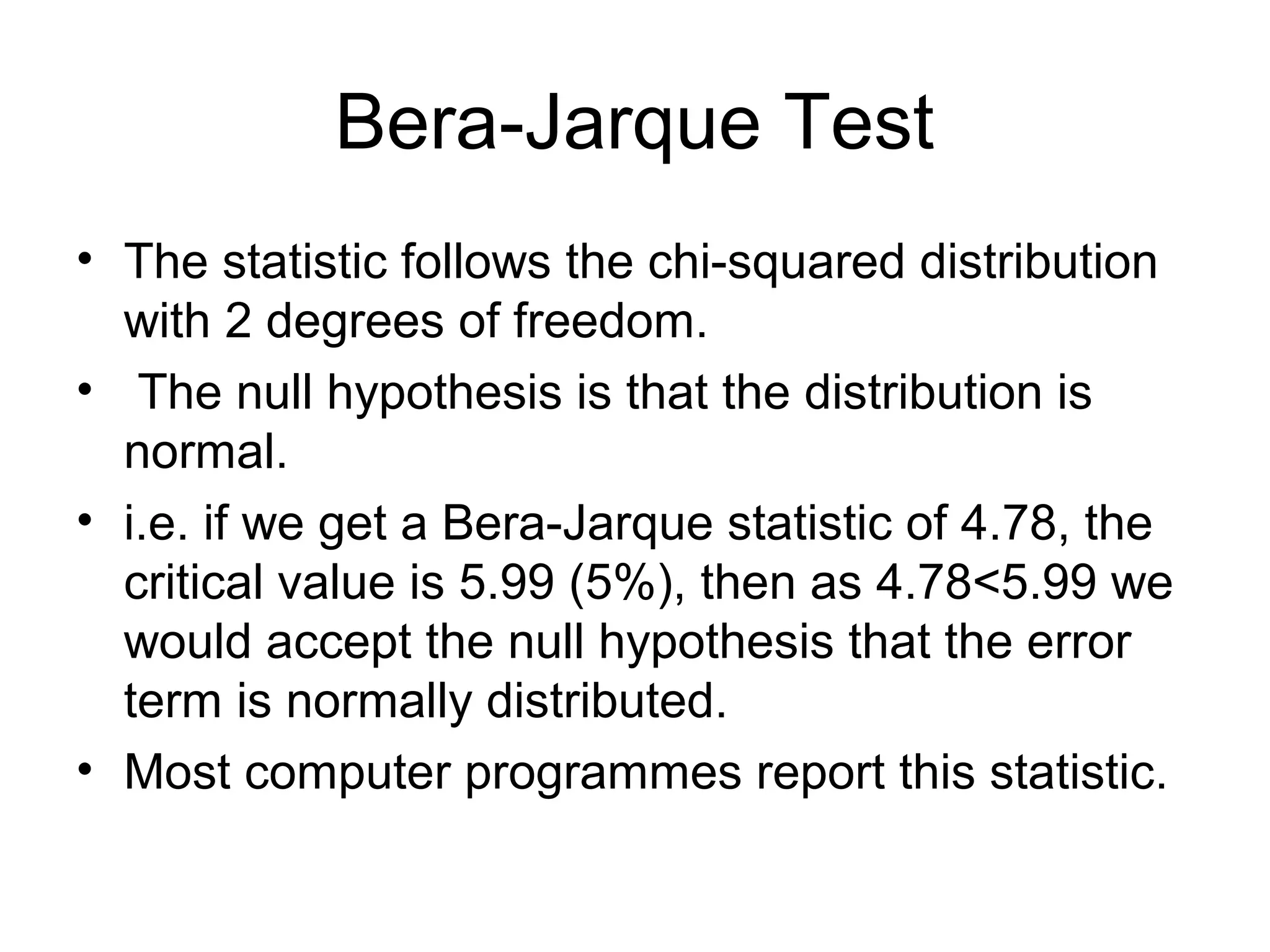
• This test for normality in effect tests for the
coefficients of skewness and excess kurtosis
being jointly equal to 0
nsobservatioofnumber
kurtosisexcessoftcoefficien
skewnessoftcoefficien
]
24
)3(
6
[
2
1
2
2
2
1
−
−
−
−
+=
T
b
b
bb
TW
Bera-Jarque Test
• The statistic follows the chi-squared distribution
with 2 degrees of freedom.
• The null hypothesis is that the distribution is
normal.
• i.e. if we get a Bera-Jarque statistic of 4.78, the
critical value is 5.99 (5%), then as 4.78<5.99 we
would accept the null hypothesis that the error
term is normally distributed.
• Most computer programmes report this statistic.
Remedies for non-normality
• The non-normality is often caused by a couple of
observations in the tails of the distribution, these
observations are often termed outliers.
• The simplest way to solve the problem is to use
a dummy variable, often called an impulse
dummy variable, which takes the value of 0,
except the one outlier observation which takes
the value of 1.
• This has the effect of forcing the residual for this
observation to 0.
• To determine where the outlier is, we could
simply plot the residuals against time.
Non-normality
• The use of this type of dummy variable is
controversial, as some argue it is an
artificial method of improving the
regression, by in effect removing the
influence of this particular observation.
• However an outlier can have an
excessively strong effect on a model,
giving an unrealistic result, so needs to be
taken into account.
Dummy Variable for Single Outlier
• In a regression of stock prices against income for
the UK, an outlier was noticed for 1992 month 9,
when the UK left the ERM. A dummy variable was
added to account for this. This produced the
following result:
.91992var1
.87.1,78.0R
(0.20)(0.23)(0.43)
80.087.067.0ˆ
2
mforiabledummyD
DW
Dys ttt
−
==
++=
Dummy Variables
• The previous set of results can be interpreted in
the usual way, in this case the dummy variable
has a significant t-statistic (4), so the outlier has
a significant effect on the regression, or put
another way the UK leaving the ERM had a
significant effect on UK stock prices.
• In many cases however the outlier will be more
difficult to interpret and may not correspond to a
particular event.
Dummy Variables
• Dummy variables are discrete variables taking a
value of ‘0’ or ‘1’. They are often called ‘on’ ‘off’
variables, being ‘on’ when they are 1.
• Dummy variables can be used either as
explanatory variables or as the dependent
variable.
• When they act as the dependent variable there
are specific problems with how the regression is
interpreted, however when they act as
explanatory variables they can be interpreted in
the same way as other variables.
Types of Explanatory Dummy
Variable
• Qualitative dummy variables: i.e. age, sex, race,
health.
• Seasonal dummy variables: depends on the
nature of the data, so quarterly data requires
three dummy variables etc.
• Dummy variables that represent a change in
policy:
– Intercept dummy variables, that pick up a change in
the intercept of the regression
– Slope dummy variables, that pick up a change in the
slope of the regression
Dummy Variables
• If y is a teachers salary and
Di = 1 if a non-smoker
Di = 0 if a smoker
We can model this in the following way:
tii uDy ++= βα
Dummy Variables
• This produces an average salary for a
smoker of E(y/Di =0) =α.
• The average salary of a non-smoker will
be E(y/Di = 1) = α + β.
• This suggests that non-smokers receive a
higher salary than smokers.
Dummy Variables
• Equally we could have used the dummy
variable in a model with other explanatory
variables. In addition to the dummy variable
we could also add years of experience (x),
to give:
tiii uxDy +++= δβα
Dummy Variables
α
α+β
Non-smoker
Smoker
y
x
Seasonal Dummy Variables
• The use of seasonal dummy variables is widespread in
finance due to the ‘day of the week’ effect on asset
prices.
• They take the same format as other dummy variables,
i.e. a January dummy variable would consist of 0, except
every observation in January which has the value of 1.
• For monthly data, we include 11 dummy variables,
quarterly data 3 etc. i.e. we have as many dummies as
months, quarters etc minus 1.
• The excluded month acts as the reference category, i.e.
all the other dummies refer to differences between
themselves and this reference month.
Seasonal Dummy variables
• If we have the following model of share prices for a
gas and electricity firm, where the share price is
regressed against 3 dummy variables. (Using
quarterly data)
tt
tt
tt
t
tt
yysQ
yysQ
yysQ
ysQ
yDDDs
80.040.580.020.060.5ˆ:4
80.090.480.070.060.5ˆ:3
80.040.480.020.160.5ˆ:2
80.060.5ˆ:1
80.020.070.020.160.5ˆ 432
+=+−=
+=+−=
+=+−=
+=
+−−−=
Seasonal Dummy variables
• The regression can not be carried out if all
the seasonal dummies are added (i.e. 4
for quarterly data), as there is perfect
multicollinearity
• Although we can use the t-test to
determine if the seasonal dummy is
significant, we usually use an F-test to
determine if they are jointly significant.
Slope Dummy Variables
• The type of dummy variable considered so far is
the intercept dummy variable, we could also use
dummy variables to model changes in the slope
of the regression line, these are known as slope
or interaction dummy variables.
• We can include either types of dummy variable
or more commonly both types in a regression, to
account for changes in the intercept and slope of
the regression line.
Slope Dummy Variables
• The slope dummy variable consists of a term
which is the product of an explanatory variable
and dummy variable (Dx):
ttt
t
ttt
t
tttttt
uxy
DWhen
uxy
DWhen
uxDxDy
++++=
=
++=
=
++++=
)()(
1
0
2110
10
2110
ββαα
βα
ββαα
Slope Dummy Variable
• Given the following results from a demand for bank
loans (bl) model, with house prices (hp) as the
explanatory variable. The dummy variable takes the
value of 0 before 1979 and 1 afterwards. The slope
dummy is going to determine the change in lending
as a result of changes to the credit laws, i.e. it is
easier to borrow based on the value of a persons
house.
18.056.012.078.0ˆ
ttttt DhphpDlb +++=
Slope Dummy variables
• We then get two separate regression lines,
before and after 1979, with different
intercepts and slope coefficients:
tt
tt
hplb
Post
hplb
e
74.090.0ˆ
:1979
56.078.0ˆ
:1979Pr
+=
−
+=
−
Test for Structural Stability
• Although the Chow test is usually used to test for
a structural break, an alternative test involving
the dummy variables can also be used.
• It involves running two regressions, one with the
dummy variables (unrestricted model) and
collecting the RSS.
• The other regression excludes the dummy
variables (restricted model) and collect this RSS.
• Use the F-test formula to produce the F-statistic
and compare with the critical values, the null
hypothesis being that the regression is
structurally stable.
The Dummy Variable Approach to
Testing for a Structural Break
• Instead of two separate regressions on each
sub-sample, as in the Chow test, we just need
the single regression with the dummy variables
(as well as without the dummy variables)
• The dummy variable approach allows us to test
a variety of hypotheses about any structural
break
• The dummy variable approach allows us to
determine if it is the intercept or slope that is
different
• Using the Chow test requires testing of sub-
samples, which reduces the degrees of freedom
Conclusion
• When running a regression, we assume the
error term is normally distributed
• The Bera-Jarque test is used to determine if the
error term is normally distributed.
• To overcome non-normality, we can use an
impulse dummy variable to account for any
outliers.
• Dummy variables have a variety of uses, mostly
being used to model qualitative effects
• Dummy variables can be in either intercept or
slope form.

Dummy variables xd

  • 1.
  • 2.
    Introduction • Discuss theuse of dummy variables in Financial Econometrics. • Examine the issue of normality and the use of dummy variables to correct any problem • Show how dummy variables affect the regression • Assess the use of intercept and slope dummy variables
  • 3.
    The Normality Assumption •In general we assume the error term is normally distributed. • Financial data often fails this assumption due to the volatile nature of the data and the numbers of outliers. • The normality of the error term can be tested using the Bera-Jarque test, which tests for the presence of skewness (non- symmetry) and kurtosis (fat tails)
  • 4.
    Bera-Jarque Test • Thistest for normality in effect tests for the coefficients of skewness and excess kurtosis being jointly equal to 0 nsobservatioofnumber kurtosisexcessoftcoefficien skewnessoftcoefficien ] 24 )3( 6 [ 2 1 2 2 2 1 − − − − += T b b bb TW
  • 5.
    Bera-Jarque Test • Thestatistic follows the chi-squared distribution with 2 degrees of freedom. • The null hypothesis is that the distribution is normal. • i.e. if we get a Bera-Jarque statistic of 4.78, the critical value is 5.99 (5%), then as 4.78<5.99 we would accept the null hypothesis that the error term is normally distributed. • Most computer programmes report this statistic.
  • 6.
    Remedies for non-normality •The non-normality is often caused by a couple of observations in the tails of the distribution, these observations are often termed outliers. • The simplest way to solve the problem is to use a dummy variable, often called an impulse dummy variable, which takes the value of 0, except the one outlier observation which takes the value of 1. • This has the effect of forcing the residual for this observation to 0. • To determine where the outlier is, we could simply plot the residuals against time.
  • 7.
    Non-normality • The useof this type of dummy variable is controversial, as some argue it is an artificial method of improving the regression, by in effect removing the influence of this particular observation. • However an outlier can have an excessively strong effect on a model, giving an unrealistic result, so needs to be taken into account.
  • 8.
    Dummy Variable forSingle Outlier • In a regression of stock prices against income for the UK, an outlier was noticed for 1992 month 9, when the UK left the ERM. A dummy variable was added to account for this. This produced the following result: .91992var1 .87.1,78.0R (0.20)(0.23)(0.43) 80.087.067.0ˆ 2 mforiabledummyD DW Dys ttt − == ++=
  • 9.
    Dummy Variables • Theprevious set of results can be interpreted in the usual way, in this case the dummy variable has a significant t-statistic (4), so the outlier has a significant effect on the regression, or put another way the UK leaving the ERM had a significant effect on UK stock prices. • In many cases however the outlier will be more difficult to interpret and may not correspond to a particular event.
  • 10.
    Dummy Variables • Dummyvariables are discrete variables taking a value of ‘0’ or ‘1’. They are often called ‘on’ ‘off’ variables, being ‘on’ when they are 1. • Dummy variables can be used either as explanatory variables or as the dependent variable. • When they act as the dependent variable there are specific problems with how the regression is interpreted, however when they act as explanatory variables they can be interpreted in the same way as other variables.
  • 11.
    Types of ExplanatoryDummy Variable • Qualitative dummy variables: i.e. age, sex, race, health. • Seasonal dummy variables: depends on the nature of the data, so quarterly data requires three dummy variables etc. • Dummy variables that represent a change in policy: – Intercept dummy variables, that pick up a change in the intercept of the regression – Slope dummy variables, that pick up a change in the slope of the regression
  • 12.
    Dummy Variables • Ify is a teachers salary and Di = 1 if a non-smoker Di = 0 if a smoker We can model this in the following way: tii uDy ++= βα
  • 13.
    Dummy Variables • Thisproduces an average salary for a smoker of E(y/Di =0) =α. • The average salary of a non-smoker will be E(y/Di = 1) = α + β. • This suggests that non-smokers receive a higher salary than smokers.
  • 14.
    Dummy Variables • Equallywe could have used the dummy variable in a model with other explanatory variables. In addition to the dummy variable we could also add years of experience (x), to give: tiii uxDy +++= δβα
  • 15.
  • 16.
    Seasonal Dummy Variables •The use of seasonal dummy variables is widespread in finance due to the ‘day of the week’ effect on asset prices. • They take the same format as other dummy variables, i.e. a January dummy variable would consist of 0, except every observation in January which has the value of 1. • For monthly data, we include 11 dummy variables, quarterly data 3 etc. i.e. we have as many dummies as months, quarters etc minus 1. • The excluded month acts as the reference category, i.e. all the other dummies refer to differences between themselves and this reference month.
  • 17.
    Seasonal Dummy variables •If we have the following model of share prices for a gas and electricity firm, where the share price is regressed against 3 dummy variables. (Using quarterly data) tt tt tt t tt yysQ yysQ yysQ ysQ yDDDs 80.040.580.020.060.5ˆ:4 80.090.480.070.060.5ˆ:3 80.040.480.020.160.5ˆ:2 80.060.5ˆ:1 80.020.070.020.160.5ˆ 432 +=+−= +=+−= +=+−= += +−−−=
  • 18.
    Seasonal Dummy variables •The regression can not be carried out if all the seasonal dummies are added (i.e. 4 for quarterly data), as there is perfect multicollinearity • Although we can use the t-test to determine if the seasonal dummy is significant, we usually use an F-test to determine if they are jointly significant.
  • 19.
    Slope Dummy Variables •The type of dummy variable considered so far is the intercept dummy variable, we could also use dummy variables to model changes in the slope of the regression line, these are known as slope or interaction dummy variables. • We can include either types of dummy variable or more commonly both types in a regression, to account for changes in the intercept and slope of the regression line.
  • 20.
    Slope Dummy Variables •The slope dummy variable consists of a term which is the product of an explanatory variable and dummy variable (Dx): ttt t ttt t tttttt uxy DWhen uxy DWhen uxDxDy ++++= = ++= = ++++= )()( 1 0 2110 10 2110 ββαα βα ββαα
  • 21.
    Slope Dummy Variable •Given the following results from a demand for bank loans (bl) model, with house prices (hp) as the explanatory variable. The dummy variable takes the value of 0 before 1979 and 1 afterwards. The slope dummy is going to determine the change in lending as a result of changes to the credit laws, i.e. it is easier to borrow based on the value of a persons house. 18.056.012.078.0ˆ ttttt DhphpDlb +++=
  • 22.
    Slope Dummy variables •We then get two separate regression lines, before and after 1979, with different intercepts and slope coefficients: tt tt hplb Post hplb e 74.090.0ˆ :1979 56.078.0ˆ :1979Pr += − += −
  • 23.
    Test for StructuralStability • Although the Chow test is usually used to test for a structural break, an alternative test involving the dummy variables can also be used. • It involves running two regressions, one with the dummy variables (unrestricted model) and collecting the RSS. • The other regression excludes the dummy variables (restricted model) and collect this RSS. • Use the F-test formula to produce the F-statistic and compare with the critical values, the null hypothesis being that the regression is structurally stable.
  • 24.
    The Dummy VariableApproach to Testing for a Structural Break • Instead of two separate regressions on each sub-sample, as in the Chow test, we just need the single regression with the dummy variables (as well as without the dummy variables) • The dummy variable approach allows us to test a variety of hypotheses about any structural break • The dummy variable approach allows us to determine if it is the intercept or slope that is different • Using the Chow test requires testing of sub- samples, which reduces the degrees of freedom
  • 25.
    Conclusion • When runninga regression, we assume the error term is normally distributed • The Bera-Jarque test is used to determine if the error term is normally distributed. • To overcome non-normality, we can use an impulse dummy variable to account for any outliers. • Dummy variables have a variety of uses, mostly being used to model qualitative effects • Dummy variables can be in either intercept or slope form.