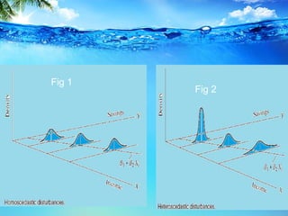
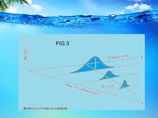
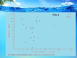
This document discusses heteroscedasticity, which occurs when the error variance is not constant. It provides examples of when the variance of errors may change, such as with income level or outliers. Graphical methods are presented for detecting heteroscedasticity by examining patterns in residual plots. Formal tests are also described, including the Park test which regresses the log of the squared residuals on explanatory variables, and the Glejser test which regresses the absolute value of residuals on variables related to the error variance. Detection of heteroscedasticity is important as it violates assumptions of the classical linear regression model.

1. HETEROSCEDASTICITY
Presented by
GEETHU RANGAN
MTECH TECHNOLOGY MANAGEMENT
DEPT OF FUTURES STUDIES
UNIVERSITY OF KERALA

2. THE NATURE OF HETEROSCEDASTICITY
• Heteroscedasticity occurs when the error
variance has non-constant variance.
• One of the important assumptions of the
classical linear regression model is that the
variance of each disturbance term ui,
conditional on the chosen values of the
explanatory variables, is some constant
number equal to σ2.

3. This is the assumption of homoscedasticity, or equal (homo) spread
(scedasticity), that is, equal variance. Symbolically,
Eu2
i = σ2 i = 1, 2, . . . , n
Fig 1

4. According to the below figure the variances ofYi are not the same. Hence, there is
heteroscedasticity.Symbolically, Eu2
i = σ2
i
Fig 2

5. • Assume that in the two-variable model
Yi = β1 + β2Xi + ui
Y represents savings and X represents income.
Figures 1 and 2 show that as income increases, savings on the average also
increase.
But in Figure 1 ,the variance of savings remains the same at all levels of
income, whereas in Figure 2 it increases with income.
It seems that in Figure 2 the higher income families on the average save
more than the lower-income families, but there is also more variability in
their savings.

6. Fig 1
Fig 2

7. Reasons why the variances of ui
may be variable
1. Following the error-learning models, as people learn, their errors of
behavior become smaller over time. In this case, σ2
i is expected to
decrease. As an example, consider Figure 3, which relates the
number of typing errors made in a given time period on a test to the
hours put in typing practice.

8. FIG 3

9. 2. As incomes grow, people have more discretionary income and hence
more scope for choice about the disposition of their income. Hence,
σ2
i is likely to increase with income. Similarly, companies with
larger profits are generally expected to show greater variability in
their dividend policies than companies with lower profits.
3. As data collecting techniques improve, σ2
i is likely to decrease. Thus,
banks that have sophisticated data processing equipment are likely to
commit fewer errors in the monthly or quarterly statements of their
customers than banks without such facilities.

10. 4. Heteroscedasticity can also arise as a result of the presence of
outliers, (either very small or very large) in relation to the
observations in the sample Figure 4.
The inclusion or exclusion of such an observation, especially if the
sample size is small, can substantially alter the results of regression
analysis. Chile can be regarded as an outlier because the given Y and
X values are much larger than for the rest of the countries. In
situations such as this, it would be hard to maintain the assumption
of homoscedasticity.

11. FIG 4

12. 5. Another source of heteroscedasticity arises from violating Assumption 9 of
CLRM, namely, that the regression model is correctly specified, very often
what looks like heteroscedasticity may be due to the fact that some important
variables are omitted from the model. But if the omitted variables are included
in the model, that impression may disappear.
6. Another source of heteroscedasticity is skewness in the distribution of one or
more regressors included in the model. Examples are economic variables such
as income, wealth, and education. It is well known that the distribution of
income and wealth in most societies is uneven, with the bulk of the income and
wealth being owned by a few at the top.

13. DETECTION OF HETEROSCEDASTICITY
Graphical Method
 If there is no a priori or empirical information about the nature of
heteroscedasticity, in practice one can do the regression analysis on
the assumption that there is no heteroscedasticity and then do an
examination of the residual squared uˆ2
i to see if they exhibit any
systematic pattern.
 Although uˆ2
i are not the same thing as u2
i , they can be used as
proxies especially if the sample size is sufficiently large..

14. An examination of the uˆ2
i may reveal
patterns such as those shown in
Figure 8. In Figure 8a we see that
there is no systematic pattern between
the two variables, suggesting that
perhaps no heteroscedasticity is
present in the data. Figure 8b to e,
however, exhibits definite patterns.
For instance, Figure 8c suggests a
linear relationship, whereas Figure 8d
and e indicates a quadratic
relationship between uˆ2
i and Yˆi.
Using such knowledge, albeit
informal, one may transform the data
in such a manner that the transformed
data do not exhibit heteroscedasticity
Fig 8
Fig 8

15.  Instead of plottinguˆ2
i against Yˆi, one may
plot them against one of the explanatory
variables Xi.
 A pattern such as that shown in Figure 9c, for
instance, suggests that the variance of the
disturbanceterm is linearly related to the X
variable.Thus, if in the regressionof savings
on income one finds a pattern such as that
shown in Figure 9c, it suggests that the
heteroscedasticvariance may be proportional
to the value of the income variable.This
knowledge may help us in transformingour
data in such a manner that in the regressionon
the transformeddata the variance of the
disturbanceis homoscedastic.
Fig 9

16. Formal Methods
 Park Test. Park suggests that σ2
i is some function of the explanatory
variable Xi. The functional form he suggested was
σ2
i = σ2Xβ
i evi
or
ln σ2
i = ln σ2 + β ln Xi + vi
(eqn 1)
 where vi is the stochastic disturbance term. Since σ2
i is generally not
known, Park suggests using uˆ2
i as a proxy and running the following
regression:
ln uˆ2
i = ln σ2 + β ln Xi + vi = α + β ln Xi + vi (eqn 2)

17. • If β turns out to be statistically significant, it would suggest that
heteroscedasticity is present in the data.
• If it turns out to be insignificant, we may accept the assumption of
homoscedasticity.
• The Park test is a two stage procedure. In the first stage we run the OLS
regression disregarding the heteroscedasticity question. We obtain uˆi
from this regression, and then in the second stage we run the regression
eqn 2

18. • Glejser Test. Test is similar in spirit to the Park test. After obtaining theresiduals uˆi from the
OLS regression,Glejser suggests regressing the absolute values of uˆi on the X variable that is
thought to be closely associated withσ2
i . In his experiments, Glejser used the following
functional forms: where vi is the error term.