Downloaded 129 times

![Laplace Transform of
unit-step Function
∞
∞ X (σ + jω ) = ∫ e −(σ + jω ) t dt
X (ω ) = ∫ x(t )e − j ωt
dt 0
−∞ 1
∞
X (σ + jω ) = − [e −(σ + jω ) t ]tt =∞
=0
σ + jω
X (ω ) = ∫ 1⋅ e − jωt dt
0 1
X (σ + jω ) = − [ 0 − e − (σ + j ω ) 0 ]
σ + jω
∞
X (ω ) = ∫ e e −σt − jωt
dt X (σ + jω ) =
1
−∞
σ + jω
∞
X (ω ) = ∫ e −(σ + jω ) t dt σ + jω → s
0
1
X ( s) =
s
INC212 Signals and Systems : 2 / 2554 Chapter 3 The Laplace Transform](https://image.slidesharecdn.com/chapter3-laplace-120427082631-phpapp01/85/Chapter3-laplace-2-320.jpg)
![Laplace Transform of Signals
∞ 1, t ≥ 0
X ( s ) = ∫ x(t )e dt − st
x(t ) = u (t ) =
0 0, t < 0
∞ ∞
L[u (t )] = ∫ u (t )e dt − st
= ∫ (1)e − st dt
−∞ 0
− st ∞
e 1
=− = −0 − (− ), s > 0
s 0
s
1
∴ L[u (t )] = , s > 0
s
INC212 Signals and Systems : 2 / 2554 Chapter 3 The Laplace Transform](https://image.slidesharecdn.com/chapter3-laplace-120427082631-phpapp01/85/Chapter3-laplace-4-320.jpg)
![Relationship between the FT and ℒ T
One-side transform or Forward transform
x(t ) = 0; t < 0 ∴ s = jω ; σ = 0
∞ ∞
X (ω ) = ∫ x(t )e − jω t
dt X ( s ) = ∫ x(t )e − st dt
0 0
X (ω ) = X ( s ) s = jω
x(t ) ↔ X ( s )
X ( s) = L[ x(t )] ; x(t ) = L−1[ X ( s )]
INC212 Signals and Systems : 2 / 2554 Chapter 3 The Laplace Transform](https://image.slidesharecdn.com/chapter3-laplace-120427082631-phpapp01/85/Chapter3-laplace-5-320.jpg)
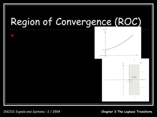
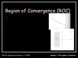
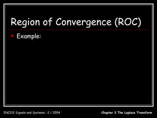
![Region of Convergence (ROC)
Example:
x(t ) = e − t u (t ) + e −2t u (t )
L ∞ ∞
x(t ) ↔ X ( s ) = ∫ [e u (t ) + e u (t )]e dt = A∫ [e −( s +1) t + e −( s + 2) t ]dt
−t − 2t − st
−∞ 0
1 1
∴ X (s) = + σ > −1
s +1 s + 2
INC212 Signals and Systems : 2 / 2554 Chapter 3 The Laplace Transform](https://image.slidesharecdn.com/chapter3-laplace-120427082631-phpapp01/85/Chapter3-laplace-9-320.jpg)
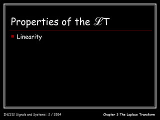
![Properties of the ℒT
Example: Linearity L[u (t ) + e − t u (t )]
1 −t 1
u (t ) ↔ and e u (t ) ↔
s s +1
−t 1 1
u (t ) + e u (t ) ↔ +
s s +1
−t 2s + 1
u (t ) + e u (t ) ↔
s ( s + 1)
INC212 Signals and Systems : 2 / 2554 Chapter 3 The Laplace Transform](https://image.slidesharecdn.com/chapter3-laplace-120427082631-phpapp01/85/Chapter3-laplace-12-320.jpg)


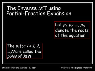
![Distinct Poles
c1 c2 cN
X ( s) = + ++
s − p1 s − p2 s − pN
ci = [( s − pi ) X ( s )]s = pi , i = 1,2, , N
x(t ) = c1e p1t
+ c2 e p2t
+ + cN e pN t
, t≥0
INC212 Signals and Systems : 2 / 2554 Chapter 3 The Laplace Transform](https://image.slidesharecdn.com/chapter3-laplace-120427082631-phpapp01/85/Chapter3-laplace-18-320.jpg)
![Example: Distinct Poles
s+2 ci = [( s − pi ) X ( s )]s = pi , i = 1,2, , N
X ( s) = 3
s + 4 s 2 + 3s s+2 2
A( s ) = s + 4 s + 3s = s ( s + 1)( s + 3) c1 = [ sX ( s )]s =0 = ( s + 1)( s + 3)
3 2 =
3
s =0
A( s ) = 0 = s ( s + 1)( s + 3)
s+2 1
p1 = 0, p2 = −1, p3 = −3 c2 = [( s + 1) X ( s )]s = −1 = =
s ( s + 3) s = −1 − 2
c1 c2 c3
X ( s) = + + s+2 −1
s − 0 s − (−1) s − (−3) c3 = [( s + 3) X ( s )]s = −3 = =
s ( s + 1) s = −3 6
c c c
X ( s) = 1 + 2 + 3 2 1 − t 1 − 3t
s s +1 s + 3 x(t ) = − e − e , t ≥ 0
3 2 6
INC212 Signals and Systems : 2 / 2554 Chapter 3 The Laplace Transform](https://image.slidesharecdn.com/chapter3-laplace-120427082631-phpapp01/85/Chapter3-laplace-19-320.jpg)

![Example: Distinct Poles with 2 or
More Poles Complex
ci = [( s − pi ) X ( s)]s = p , i = 1,2,, N
s − 2s + 1
2 i
X (s) = 3 s 2 − 2s + 1
s + 3s 2 + 4 s + 2 c1 = [( s + 1 − j ) X ( s )]s =−1+ j =
( s + 1 + j )( s + 1) s =−1+ j
A( s ) = s 3 + 3s 2 + 4 s + 2
= ( s + 1 − j )( s + 1 + j )( s + 1) −3
c1 = + j2
2
p1 = −1 + j , p2 = −1 − j , p3 = −1
9 5
c1 = +4 = ;
X ( s) =
c1
+
c1
+
c3 4 2
s − (−1 + j ) s − (−1 − j ) s − (−1) −4
∠c1 = 180° + tan −1 = 126.87°
c1 c1 c3 3
X ( s) = + +
s +1− j s +1+ j s +1 s 2 − 2s + 1
c3 = [( s + 1) X ( s )]s = −1 = 2 =4
s + 2 s + 2 s = −1
x(t ) = 5e −t cos(t + 126.87°) + 4e − t , t ≥ 0
INC212 Signals and Systems : 2 / 2554 Chapter 3 The Laplace Transform](https://image.slidesharecdn.com/chapter3-laplace-120427082631-phpapp01/85/Chapter3-laplace-21-320.jpg)
![Repeated Poles
B( s) c c2 cr c cN
X (s) = X ( s) = 1 + ++ + r +1 + +
A( s ) s − p1 ( s − p1 ) 2 ( s − p1 ) r s − pr +1 s − pN
ci = [( s − pi ) X ( s )]s = pi , i = r + 1, r + 2, , N
cr = [( s − p1 ) r X ( s )]s = p1
1d
i = 1,2, , r − 1 i = 1; cr −1 = [( s − p1 ) r X ( s )]
1! ds
s = p1
1 di
cr − i = i [( s − p1 ) X ( s )]
r
1 d2
i! ds s = p1 i = 2; cr − 2 = 2 [( s − p1 ) r X ( s )]
2! ds s= p 1
x(t ) = c1e p1t + c2te p1t + + cr t r −1e p1t + cr +1e pr +1t + + c N e p N t , t ≥ 0
INC212 Signals and Systems : 2 / 2554 Chapter 3 The Laplace Transform](https://image.slidesharecdn.com/chapter3-laplace-120427082631-phpapp01/85/Chapter3-laplace-22-320.jpg)
![Example: Repeated Poles
5s − 1 c1 c2 c
X (s) = 3 X (s) = + + 3
s − 3s − 2 s + 1 ( s + 1) 2 s − 2
1d d 5s − 1 −9
c1 = [( s + 1) 2 X ( s )] = [ ] = = −1
1! ds
s = −1 ds s − 2 s = −1 ( s − 2)
2
s = −1
5s − 1
c2 = [( s + 1) 2 X ( s )]s = −1 = =2
s − 2 s = −1
5s − 1
c3 = [( s − 2) X ( s )]s = 2 = =1
( s + 1) 2 s =2
x(t ) = −e − t + 2te − t + e 2t , t ≥ 0
INC212 Signals and Systems : 2 / 2554 Chapter 3 The Laplace Transform](https://image.slidesharecdn.com/chapter3-laplace-120427082631-phpapp01/85/Chapter3-laplace-23-320.jpg)
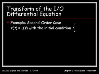
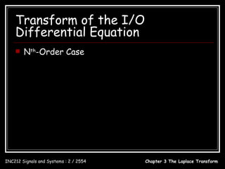
![Transform of the I/O
Differential Equation
Second-Order Case
d 2 y (t ) dy (t ) dx(t )
2
+ a1 + a0 y (t ) = b1 + b0 x(t )
dt dt dt
[ ]
s 2Y ( s ) − y (0 − ) s − y (0 − ) + a1 sY ( s ) − y (0 − ) + a0Y ( s ) = b1sX ( s ) + b0 X ( s )
y (0 − ) s + y (0 − ) + a1 y (0 − )
b1s + b0
Y (s) = + 2 X ( s)
s + a1s + a0
2
s + a1s + a0
If initial condition = 0 :
b1s + b0 b1s + b0
Y (s) = 2 X ( s) ; H ( s) = 2
s + a1s + a0 s + a1s + a0
INC212 Signals and Systems : 2 / 2554 Chapter 3 The Laplace Transform](https://image.slidesharecdn.com/chapter3-laplace-120427082631-phpapp01/85/Chapter3-laplace-28-320.jpg)
![Transform of the I/O
Convolution Integral
Example: Determining the TF
y (t ) = 2 − 3e −t + e −2t cos 2t , t ≥ 0 2 3 s+2
− +
2 3 s+2 s s + 1 ( s + 2) 2 + 4
Y (s) = − + H (s) =
s s + 1 ( s + 2) + 4 2 1
s +1
1 2( s + 1) ( s + 1)( s + 2)
X (s) = = −3+
s +1 s ( s + 2) 2 + 4
[2( s + 1) − 3s ][( s + 2) 2 + 4] + s ( s + 1)( s + 2)
=
s[( s + 2) 2 + 4]
s 2 + 2s + 16
= 3
s + 4 s 2 + 8s
INC212 Signals and Systems : 2 / 2554 Chapter 3 The Laplace Transform](https://image.slidesharecdn.com/chapter3-laplace-120427082631-phpapp01/85/Chapter3-laplace-33-320.jpg)

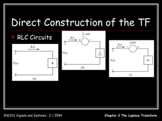
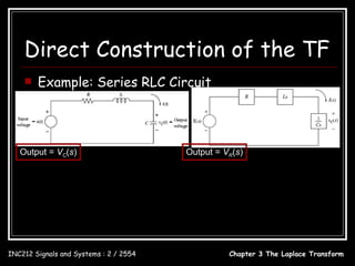
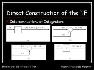
![Direct Construction of the TF
sQ1 ( s) = −4Q1 ( s ) + X ( s)
Example: Q1 ( s) =
1
s+4
X (s)
sQ2 ( s ) = Q1 ( s) − 3Q2 ( s) + X ( s )
1
Q2 ( s ) = [Q1 ( s ) + X ( s )]
s+3
1 1
= + 1 X ( s )
s +3 s +4
s+5
= X ( s)
( s + 3)( s + 4)
Y ( s ) = Q2 ( s ) + X ( s )
s+5
= X ( s) + X ( s)
( s + 3)( s + 4)
s 2 + 8s + 17
= X ( s)
( s + 3)( s + 4)
s 2 + 8s + 17 s 2 + 8s + 17
H ( s) = =
( s + 3)( s + 4) s 2 + 7 s + 12
INC212 Signals and Systems : 2 / 2554 Chapter 3 The Laplace Transform](https://image.slidesharecdn.com/chapter3-laplace-120427082631-phpapp01/85/Chapter3-laplace-45-320.jpg)
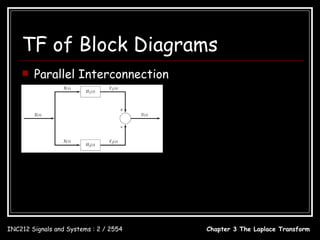
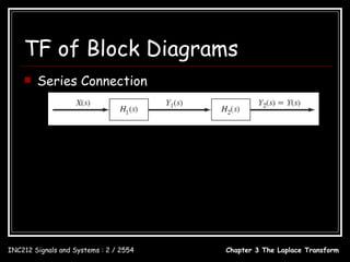
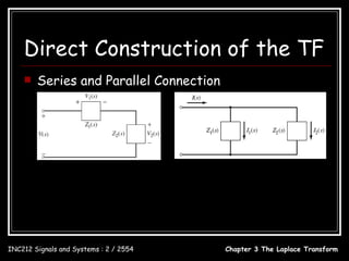
![TF of Block Diagrams
Feedback Connection Y ( s) = H1 ( s) X 1 ( s)
X 1 ( s ) = X ( s ) − Y2 ( s )
= X ( s ) − H 2 ( s )Y ( s )
Y ( s ) = H1 ( s )[ X ( s ) − H 2 ( s )Y ( s )]
H1 ( s )
Y (s) = X (s)
1 + H1 ( s) H 2 ( s)
H1 ( s)
H (s) =
1 + H1 ( s) H 2 ( s)
H1 ( s)
H (s) =
1 − H1 ( s ) H 2 ( s )
INC212 Signals and Systems : 2 / 2554 Chapter 3 The Laplace Transform](https://image.slidesharecdn.com/chapter3-laplace-120427082631-phpapp01/85/Chapter3-laplace-48-320.jpg)

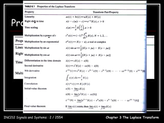
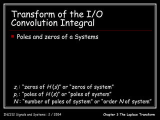
The document summarizes key concepts about the Laplace transform. It defines the Laplace transform, discusses properties like linearity and time shifting. It provides examples of taking the Laplace transform of unit step functions. It also covers computing the inverse Laplace transform using partial fraction expansion and handling cases with repeated or complex poles.


![Circuit Network Analysis - [Chapter4] Laplace Transform](https://cdn.slidesharecdn.com/ss_thumbnails/ch4-150613063858-lva1-app6891-thumbnail.jpg?width=640&height=640&fit=bounds)


![Mathematics of nyquist plot [autosaved] [autosaved]](https://cdn.slidesharecdn.com/ss_thumbnails/mathematicsofnyquistplotautosavedautosaved-150219123133-conversion-gate02-thumbnail.jpg?width=640&height=640&fit=bounds)


![11.[95 103]solution of telegraph equation by modified of double sumudu transf...](https://cdn.slidesharecdn.com/ss_thumbnails/11-95-103solutionoftelegraphequationbymodifiedofdoublesumudutransformelzakitransform-120513000213-phpapp01-thumbnail.jpg?width=640&height=640&fit=bounds)