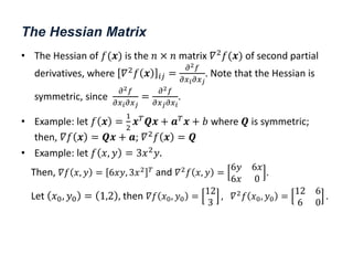
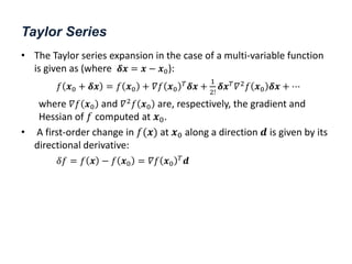
This document provides an overview of an optimization methods course, including its objectives, prerequisites, and materials. The course covers topics such as linear programming, nonlinear programming, and mixed integer programming problems. It also includes mathematical preliminaries on topics like convex sets and functions, gradients, Hessians, and Taylor series expansions. Methods for solving systems of linear equations and examples are presented.


![Function Definitions
• Continuous Function. A function 𝑓(𝒙) is continuous at a point 𝒙0 if
lim
𝒙→𝒙0
𝑓(𝒙) = 𝑓(𝒙0).
• Affine Function. The function 𝑓 𝒙 = 𝒂𝑇𝒙 + 𝑏 is affine.
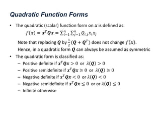
• Quadratic Function. A quadrative function is of the form:
𝑓 𝒙 =
1
2
𝒙𝑇𝑸𝒙 + 𝒂𝑇𝒙 + 𝑏, where 𝑸 is symmetric.
• Convex Functions. A function 𝑓(𝒙) defined on a convex set 𝑆 is
convex if and only if for every pair 𝒙, 𝒚 ∈ 𝑆,
𝑓 𝛼𝒙 + 1 − 𝛼 𝒚 ≤ 𝛼𝑓 𝒙 + 1 − 𝛼 𝑓 𝒚 , 𝛼 ∈ [0,1]
– Affine functions defined over convex sets are convex.
– Quadratic functions defined over convex sets are convex only if
𝑸 > 0, i.e., all its eigenvalues are positive.](https://image.slidesharecdn.com/optimumengineeringdesign-day2b-240221200552-857f4f04/85/Optimum-Engineering-Design-Day-2b-Classical-Optimization-methods-8-320.jpg)


![[Convex Optimization_slides Stephen Boyd] S.Boyd L.Vandenberghe .pdf](https://cdn.slidesharecdn.com/ss_thumbnails/convexoptimizationslidesstephenboyds-260110114011-5c7e91dc-thumbnail.jpg?width=640&height=640&fit=bounds)