1) Jordan's lemma is used to convert real integrals over the infinite real axis into complex integrals over a contour enclosing the real axis in the complex plane. 2) Several examples are provided of using residues and Jordan's lemma to evaluate definite integrals over the real line or infinite intervals that involve functions with poles, including integrals of x^2, sin(x)/x, 1/(x^2+a^2)^2, and sin(x)/(x(x^2+a^2)). 3) The technique involves closing the contour with a semicircle at infinity where the integral over the semicircle goes to zero by Jordan's lemma, leaving the original integral equal to the residue theorem applied to the

1. NPTEL – Physics – Mathematical Physics - 1
Lecture 38
Jordon’s lemma
∞
We need to convert real integrals of the form ∫ 𝑓(𝑥)𝑑𝑥 into a
complex integral by
−∞
joining ends of the real axis by a semi circle at infinity in the upper or lower
half plane. It
is useful to consider
J(𝑅, 𝑎) = ∫ 𝑒𝑖𝑎𝑧𝑔(𝑧)𝑑𝑧
𝐼𝑅
𝑎 > 0
𝛤𝑅 is the semicircle of radius R in the upper plane. We need 𝑔(𝑧) to be continuous such
that 𝑔(𝑅𝑒𝑖𝜃) → 0 as 𝑅 → ∞ for 0 ≤ 𝜃 ≤ 𝜋.
𝐿𝑖𝑚| 𝐽(𝑅, 𝑎)| = 0 ⇒ called as Jordon’s lemma
𝑅→∞
Calculations of definite Integrals
∞
∫
𝐹(𝑥)𝑑𝑥
−∞
See that this is a real integral a integration over a real line. One can mimic the ±∞ limits
by including over ±𝑅 and − 𝑅 → ∞. This is of course accompanied by a curve 𝛤 taken in
the positive sense.
Joint initiative of IITs and IISc – Funded by MHRD Page 37 of 66

2. NPTEL – Physics – Mathematical Physics - 1
Example. ∫
𝑥2𝑑𝑥
−∞ (𝑥2+1)2(𝑥2+2𝑥+2)
∞
Change 𝑥 → 𝑧
The poles of
𝑧2
(𝑧2+1)2(𝑧2+2𝑧+2)
enclosed by 𝐶 are 𝑧 = 𝑖 of order 2 and
𝑧 = −1 + 𝑖 is of order 1.
Residue at 𝑧 = −1 + 𝑖 (the other pole is not
included)
𝐿𝑖𝑚 (𝑧 + 1 − 𝑖)
𝑧→−1+𝑖
𝑧2
(𝑧2+1(𝑧+1−𝑖)(𝑧+1+𝑖) 50
= 3−4𝑖
Thus, ∮
𝑧2𝑑𝑧
𝑐 (𝑧2+1)2(𝑧2+2𝑧
+2)
= 2𝜋𝑖 ( + ) =
9𝑖−12 3−4𝑖
100 25
7𝜋
50
𝑅
∫
−
𝑅
𝑥2𝑑𝑥
(𝑥2 + 1)2(𝑥2 + 2𝑥 + 2)
+ ∫
Γ
𝑧2𝑑𝑧
(𝑧2 + 1)2(𝑧2 + 2𝑧 + 2) 50
=
7𝜋
As 𝑅 → ∞, the second integral tends to zero by Jordan’s lemma.
Example 2. ∫
2𝜋 𝑑𝜃
𝑎+𝑏𝑠𝑖𝑛
𝜃
𝑎 > 𝑏
0
𝑧 = 𝑒𝑖𝜃 , 𝑠𝑖𝑛𝜃 = 𝑒𝑖𝜃 − 𝑒−𝑖𝜃
2𝑖
=
𝑧 −
1
𝑧
2𝑖
𝑑𝑧 = 𝑖𝑒𝑖𝜃 𝑑𝜃 = 𝑖𝑧𝑑𝜃
2𝜋
∫
0
𝑑𝜃
𝑎 + 𝑏𝑠𝑖𝑛𝜃
= ∮
𝑐
𝑑𝑧⁄𝑖
𝑧
𝑎 + 𝑏 (𝑧 − 1
)
𝑧 ⁄
2𝑖
= ∮ 2𝑑𝑧
𝑐 𝑏𝑧2+2𝑎𝑖𝑧−𝑏
Joint initiative of IITs and IISc – Funded by MHRD Page 38 of 66

3. NPTEL – Physics – Mathematical Physics - 1
where 𝐶 is a circle of unit radius with center at the origin. The poles of
obtained by solving, 𝑏𝑧2 + 2𝑎𝑖𝑧 − 𝑏 = 0
2
𝑏𝑧2+2𝑎𝑖𝑧−𝑏 are
𝑧 =
−𝑎 + √𝑎2 − 𝑏2 −𝑎 − √𝑎2 − 𝑏2
𝑏 𝑏
𝑖, 𝑖
(i) (ii)
Suppose the value of a and b are such that Only (i) lies within 𝐶, then the
Residue at 𝑧1 𝐿𝑖𝑚(𝑧 − 𝑧1)
𝑧→𝑧1
2
𝑏𝑧2+2𝑎𝑖𝑧−𝑏
Using L’hospital’s rule.
𝐿𝑡 =
𝑧→𝑧1 2𝑏𝑧 + 2𝑎𝑖 𝑏𝑧1 + 𝑎𝑖
2 1
=
1
√𝑎2 − 𝑏2𝑖
Thus, ∮
2𝑑𝑧
𝑏𝑧2+2𝑎𝑖𝑧−𝑏 = 2𝜋𝑖 (
1
√𝑎2−𝑏2𝑖 )
= 2𝜋
√𝑎2−𝑏2
Example 3. ∫
𝑑𝜃
(5+3𝑠𝑖𝑛𝜃
)2
2𝜋
0
Using ∫
2𝜋 𝑑𝜃
𝑎+𝑏𝑠𝑖𝑛𝜃 √𝑎2−𝑏2
0
= (𝑎 > 𝑏)
2𝜋
Differentiating both sides with respect to a (keeping b as constant)
𝑑 𝑑𝜃
𝑑𝑎 𝑎 + 𝑏𝑠𝑖𝑛𝜃
0
∫
2𝜋
= − ∫
0
𝑑𝜃 𝑑 2𝜋
(𝑎 + 𝑏𝑠𝑖𝑛𝜃)2 𝑑𝑎
2𝜋
= (
√𝑎2 − 𝑏2
) =
2𝜋𝑎
(𝑎2 − 𝑏2)1⁄2
Here 𝑎 = 5 and
2𝜋
𝑏 = −3
∫
0
𝑑𝜃
(5 − 3𝑠𝑖𝑛𝜃)2
=
10𝜋
3
(25 − 9) ⁄2
=
5𝜋
32
Joint initiative of IITs and IISc – Funded by MHRD Page 39 of 66

4. NPTEL – Physics – Mathematical Physics - 1
Example 4. Find ∫ 𝑥2+1
∞ 𝑐𝑜𝑠𝑚𝑥
0
𝑑𝑥
Consider another integral ∮
𝑒𝑖𝑚
𝑧
𝑐 𝑧
2+1
𝑑𝑧 where
The integral has simple poles at 𝑧 = ±𝑖, but only 𝑧 = +𝑖 lies within 𝐶.
Residue at 𝑧 = 𝑖 is 𝐿𝑖𝑚 {(𝑧 − 𝑖)
𝑧→𝑖
𝑒𝑖𝑚
𝑧
(𝑧−𝑖)(𝑧+𝑖)
}
= 𝑒
−𝑚
2𝑖
∮
𝑐
𝑒𝑖𝑚
𝑧
𝑧2 + 1
𝑑𝑧 = 2𝜋𝑖 ( ) = 𝜋𝑒−𝑚
𝑒−𝑚
2𝑖
∫
𝑅 𝑐𝑜𝑠𝑚𝑥 𝑑
𝑥
−𝑅 𝑥2+1
+ 𝑖 ∫
𝑅 𝑠𝑖𝑛𝑚𝑥 𝑑
𝑥
−𝑅 𝑥2+1
+ ∫
𝑒𝑖𝑚 𝑧 𝑑
𝑧
𝑐 𝑧
2+1
= 𝜋𝑒𝑚
0 being an 0
odd function
𝑅
2 ∫
0
𝑐𝑜𝑠𝑚𝑥 𝑑𝑥
𝑥2 + 1
=
𝜋𝑒−𝑚
2
Example 5.
∞
Evaluate 𝐼 = 2 ∫
𝑑𝑥
(𝑥2+𝑎2)2
0
Answer: The integrand in an even function of 𝑥. Then we can apply,
Joint initiative of IITs and IISc – Funded by MHRD Page 40 of 66

5. NPTEL – Physics – Mathematical Physics - 1
∞ 0 ∞
∫0 𝑓(𝑧)𝑑𝑧 + ∫−∞ 𝑓(𝑧)𝑑𝑧 = ∫−∞ 𝑓(𝑧)𝑑𝑧
Graphically the contour looks like
Or
Since we are involving contours that extend in the complex plane, the integrand can be
written as,
∫
∞ 𝑑𝑧
−∞ (𝑧2+𝑎2)2 −∞ (𝑧+𝑖𝑎)2(𝑧−𝑖𝑎)2
= ∫
∞ 𝑑𝑧
; two second order poles at ±𝑖𝑎
Involving the first contour, only the pole ia is included
Residue = 𝐿𝑖𝑚
𝑧→𝑧0 (𝑗−𝑖)! 𝑑𝑧𝑗−1
1 𝑑𝑖−1
[(𝑧 − 𝑧 )𝑗𝑓(𝑧)]
0
𝐽 = 2, 𝑧0 = 𝑖𝑎, Residue = − 8 (𝑖𝑎)3
2 1
Thus, 𝐼 = 𝜋⁄2𝑎3
Involving the second contour
Residue = −
2
8 (−𝑖𝑎)3
1
Thus, 𝐼 =
𝜋 2
𝑎3
Thus the final answer is same, irrespective of the choice of the contour as it should be.
The integral over the curved part is zero using Jordan’s
lemma
Joint initiative of IITs and IISc – Funded by MHRD Page 41 of 66

6. NPTEL – Physics – Mathematical Physics - 1
Example 6.
𝑥(𝑥2+𝑎2)
∞
Evaluate 𝐼 = ∫ 𝑑𝑥
𝑠𝑖𝑛
𝑥
0
using Jordan’s lemma
Changing 𝑥 → 𝑧
∞ 𝑑𝑧𝑠𝑖𝑛𝑧
𝐼 = ∫
𝑧(𝑧2+𝑎2)
0
Again the integrand is even, So
𝐼 = 1
∫
∞ 𝑑𝑧(𝑒 −𝑒 )
2 −∞ 2𝑖𝑧(𝑧2+𝑎2)
𝑖𝑧 −𝑖𝑧
= 𝐼1 − 𝐼
2
To evaluate 𝐼1, take the contour as below, which encloses two simple poles
𝐼1 = 2 ∮ 2𝑖𝑧(𝑧2+𝑎2)
we can write it as a closed integral as the integral over 𝛤 is a zero
1 𝑑𝑧𝑒𝑖
𝑧
using Jordan’s lemma.
Residue at the origin =
1
2𝑖𝑎2
Residue at 𝑖𝑎 =
𝑒−𝑎
−4𝑖𝑎2
Thus, 𝐼1 = 𝑎2 (1 − 2
)
𝜋 𝑒−𝑎
The contour is
−∞ 0 ∞
Since there is a pole at the origin, we shall have to deform the contour. Here
Joint initiative of IITs and IISc – Funded by MHRD Page 42 of 66
𝐼1 =
2
∫
2𝑖𝑧(𝑧2 + 𝑎2)
−∞
1 𝑑𝑧𝑒𝑖𝑧
∞

7. NPTEL – Physics – Mathematical Physics - 1
𝐼2 = 2
∮ 2𝑖𝑧(𝑧+𝑖𝑎)(𝑧−𝑖𝑎)
1 𝑒−𝑖𝑧
Only one pole is enclosed at 𝑧 = −𝑖𝑎
Calculating the residue,
𝐼2 = −𝜋 ( )
𝑒−𝑎
−2𝑎2
𝜋
𝐼 = 𝐼1 − 𝐼2 =
𝑎2 (1 −
𝑒−𝑎 𝜋𝑒−𝑎
) −
2 2𝑎2
= 𝜋
(1 − 𝑒−𝑎)
𝑎2
Example 7. ∫
∞ 𝑠𝑖𝑛𝑥
𝑥
𝑑𝑥
0
As earlier, we can not integrate through a singularity, we modify the contour by indenting
the path at 𝑧 = 0.
Since 𝑧 = 0 is outside the region of integration.
𝑧
∮ 𝑑𝑧 = 0
𝑒𝑖
𝑧
𝑐
Joint initiative of IITs and IISc – Funded by MHRD Page 43 of 66

8. NPTEL – Physics – Mathematical Physics - 1
−𝜖
∫
𝑒𝑖𝑥 𝑑𝑥
𝑥 𝑧 𝑥
+ ∫ 𝑑𝑧 + ∫ 𝑑𝑥 +
𝑒𝑖
𝑧
𝐻𝐽 𝐴 𝜖
𝑒𝑖𝑥
𝑅
∫
𝐵𝐷𝐸𝐹
𝐺
𝑒𝑖
𝑧
𝑧
𝑑𝑧 = 0
Replacing 𝑥 → −𝑥 in the first integral and continuing with the third integral,
∫
𝑅 𝑒𝑖𝑥−𝑒−𝑖𝑥 𝑒𝑖𝑧
𝜖 𝑥 𝐻𝐽 𝐴
𝑧
+ ∫ 𝑑𝑧 + ∫
𝑒𝑖
𝑧
𝐵𝐷𝐸𝐹𝐺 𝑧
𝑑𝑧 = 0
𝑅 𝑠𝑖𝑛𝑥 𝑒
Thus, 2𝑖 ∫ = − ∫ 𝑑𝑧
− ∫ 𝑑𝑧
𝜖 𝑥 𝐻𝐽 𝐴 𝑧 𝐵𝐷𝐸𝐹𝐺 𝑧
𝑖
𝑧
𝑒𝑖
𝑧
Let 𝜖 → 0, 𝑅 → ∞, the second integral on the RHS approaches zero. For the first one,
𝑧 = 𝜖𝑒𝑖𝜃, 𝑑𝑧 = 𝑖𝜖𝑒𝑖𝜃𝑑𝜃
−𝐿𝑖𝑚 ∫
𝜖→0
𝜋
𝑒𝑖𝜖𝑒𝑖
𝜃
𝜖𝑒𝑖𝜃
0 0
𝑖𝜖𝑒𝑖𝜃𝑑𝜃 = − 𝐿𝑖𝑚 ∫ 𝑖𝑒𝑖𝜖𝑒𝑖𝜃
𝑑𝜃
𝜖→0
𝜋
= 𝜋𝑖
𝑅 𝑠𝑖𝑛𝑥
Thus, 𝐿𝑖𝑚 2𝑖 ∫
𝑑𝑥 = 𝜋𝑖
𝑅→∞ 𝜖 𝑥
𝜖→0
∞
𝑊, ∫
0
𝑠𝑖𝑛𝑥
𝑥
𝑑𝑥 =
𝜋
2
Example. 8. ∫
∞ 𝑥𝑝−1
0 1+𝑥
𝑑𝑥 𝑜 < 𝑝 < 1
Consider ∮
𝑧𝑝−1
𝐶 1+𝑧
𝑑𝑧 𝑧 = 0 is a branch point. So choose a contour such as,
Joint initiative of IITs and IISc – Funded by MHRD Page 44 of 66

9. NPTEL – Physics – Mathematical Physics - 1
The real positive x-axis is the branch cut where AB and GH coincide, but are given a
width for visual purposes. Also the integrand has a simple pole
𝑧 = −1 inside C.
Residue at 𝑧 = −1 = 𝑒𝑖𝜋 is
𝐿𝑖𝑚 (𝑧 + 1)
𝑧→−1
𝑧𝑝−1
1 + 𝑧
= (𝑒𝑖𝜋)𝑝−1 = 𝑒(𝑝−1)𝑖𝜋
Then, ∮ 𝑧𝑝−1
1+𝑧
𝑑𝑧 = 2𝜋𝑖𝑒(𝑝−1)𝜋𝑖
∫ + ∫
𝐴𝐵 𝐵𝐷𝐸𝐹𝐺
+ ∫ + ∫
𝐺𝐻 𝐻𝐽𝐴
= 2𝜋𝑖𝑒(𝑝−1)𝜋𝑖
Thus, ∫
𝑅 𝑥𝑝−1
𝜖 1+𝑥 0 1+𝑅𝑒𝑖 𝜃 1+𝑥𝑒2𝜋
𝑖
𝑑𝑥 + ∫ + ∫
2𝜋 (𝑅𝑒𝑖𝜃)𝑝−1𝑖𝑅𝑒𝑖𝜃𝑑𝜃 𝜖 (𝑥𝑒2𝜋𝑖)𝑝−1
𝑅
𝑑𝑥 + ∫ 1+𝜖𝑒𝑖
𝜃
0 (𝜖𝑒𝑖𝜃)𝑝−1𝑖𝜖𝑒𝑖𝜃𝑑𝜃
2𝜋
= 2𝜋𝑒(𝑝−1)𝜋𝑖
as 𝜖 → 0, 𝑅 → 𝛼, second and fourth integral are zero.
Hence
∞
∫
0
𝑥𝑝−1
1 + 𝑥
0
𝑑𝑥 + ∫
∞
𝑒2𝜋𝑖(𝑝−1)𝑥𝑝−1
1 + 𝑥
𝑑𝑥 = 2𝜋𝑒(𝑝−1)𝜋𝑖
⇒ (1 − 𝑒2𝜋𝑖(𝑝−1)) ∫
𝑥
𝑑𝑥 = 2𝜋𝑖𝑒(𝑝−1)𝜋𝑖
𝑝−1
1 + 𝑥
∞
0
∞
∫
0
𝑥𝑝−1
1 + 𝑥
𝑑𝑥 =
2𝜋𝑖𝑒(𝑝−1)𝜋𝑖
1 − 𝑒2𝜋𝑖(𝑝−1)
Joint initiative of IITs and IISc – Funded by MHRD Page 45 of 66

10. NPTEL – Physics – Mathematical Physics - 1
∞ √𝑥𝑑𝑥
Example 9. Consider the integral, I = ∫ 1+𝑥2
0
∮ √𝑧𝑑𝑧
1+𝑧2
Thus, ∮ √𝑧𝑑𝑧
= 2𝐼
1+𝑧2
Using residues,
∮ √𝑧𝑑𝑧
= 𝜋√2
1+𝑧2
𝐼 = 𝜋
√2
⁄
Analytic functions
A complex valued function 𝑓(𝑧) of a complex variable 𝑧 (= 𝑥 + 𝑖𝑦) in some
domain D of the complex plane defined as -
𝑓(𝑧) = 𝑢(𝑥, 𝑦) + 𝑖𝑣(𝑥, 𝑦)
u and v real functions of two real variables x and y. 𝑓(𝑧) is a continuous and
single valued function everywhere in the domain D. Let us take an arbitrary point 𝑧0. 𝑓 (𝑧
) is defined at the vicinity of 𝑧0. The derivative of 𝑓(𝑧) at 𝑧 = 𝑧0 is defined as,
𝑓′(𝑧0) = 𝐿𝑖𝑚
𝑧→𝑧0 𝑧 − 𝑧0
𝑓(𝑧) − 𝑓(𝑧0)
Now there are two ways to approach
increasing 𝑦 → 𝑦0. Then,
𝑧0(= 𝑥0 + 𝑖𝑦0). By keeping 𝑦0 constant and
Joint initiative of IITs and IISc – Funded by MHRD Page 46 of 66

11. NPTEL – Physics – Mathematical Physics - 1
𝑓′(𝑧0) = 𝐿𝑖𝑚 [
𝑧→𝑧0
𝑢(𝑥,𝑦0)−𝑢(𝑥0,𝑦0
𝑥−𝑥0
+ 𝑖
𝑣(𝑥,𝑦0)−𝑣(𝑥0,𝑦0
𝑥−𝑥0
]
= 𝜕𝑢
(𝑥 𝑦 ) + 𝑖 𝜕𝑣
(𝑥 , 𝑦 )
𝜕𝑥 𝜕𝑥
0, 0 0 0
Similarly
𝑓′(𝑧0) = 𝐿𝑖𝑚 [
𝑧→𝑧0
𝑢(𝑥0,𝑦)−𝑢(𝑥0,𝑦0
𝑖(𝑦−𝑦0)
+ 𝑖
𝑣(𝑥0,𝑦)−𝑣(𝑥0,𝑦0)
𝑖(𝑦−𝑦0)
]
= −𝑖 𝜕𝑢
(𝑥 , 𝑦 ) + 𝜕𝑣
(𝑥 , 𝑦 )
𝜕𝑦 𝜕𝑦
0 0 0 0
But the order of differentiation should not matter
𝜕𝑢
= 𝜕
𝑣
𝜕𝑥 𝜕𝑦
𝜕𝑣
= − 𝜕𝑢
𝜕𝑥 𝜕𝑦
More on multiple valued
functions
Consider a function, 𝑧 ⁄2.
At each point 𝑧 = 𝑟𝑒𝑖𝜃. Thus it can attain two possible values,
1
𝑧 = 𝑟 𝑒𝑥𝑝 [
1 1
2 2
⁄ ⁄ 𝑖(𝜃 + 2𝑘𝜋)
2
⁄ ] , 𝑘 = 0,1
Thus it is a double valued function. The two values of k correspond to two
different
1
branches of 𝑧2 .
For some reasons, it may be required to restrict the function to either of the branches. The
problem arises when one tries to traverse along a closed loop.
Joint initiative of IITs and IISc – Funded by MHRD Page 47 of 66

12. NPTEL – Physics – Mathematical Physics - 1
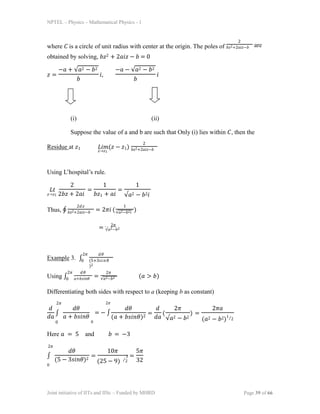
Consider 𝑘 = 0 branch. Starting from a point 𝑧0 = 𝑟0𝑒𝑖𝜃0 , let’s move around the contour
𝐶. When we come back to the starting point by changing 𝜃0 → 𝜃0 + 2𝜋, the final value of
the function is √𝑟0𝑒
𝑖(𝜃0+2𝜋⁄2 which actually corresponds to 𝑘 = 1 branch. Thus we
change branch for the reason 𝐶 encloses origin. Thus the origin, 𝑧 = 0 is called a branch
point. Also the point at infinity is also a branch point. Thus joining two branch points, we
get the branch cut. We are not allowed to cross this line in order to have single-
valuedness of the function. Thus the functions are
𝑔1(𝑧) = √𝑟 𝑒 ⁄2 and 𝑔2(𝑧) = √𝑟 𝑒
for 0 < 𝜃 < 2𝜋 and 𝑟 > 0
𝑖𝜃 𝑖(𝜃+2𝜋
)
⁄2
Now one can check that the functions 𝑔1(𝑧) and 𝑔2(𝑧) are analytic. (use CR condition to
check)
Example 10.
Find the branch points of the following functions and construct suitable branch
cuts.
(a) [(𝑧 − 1)(𝑧 + 𝑖)]1⁄2, (𝑏) (𝑧 +4
)
Joint initiative of IITs and IISc – Funded by MHRD Page 48 of 66
2
𝑧+1
1⁄2
(a) The branch points are at 𝑧 = 1 and 𝑧 = −𝑖
To see this, let 𝑧 – 1 = 𝑟1𝑒𝑖𝜃1 and 𝑧 + 𝑖 = 𝑟2𝑒𝑖𝜃2 and try encircling in closed paths.
For example after moving around 𝑧 = 1, 𝜃1 changes by 2𝜋 but 𝜃2 returns to the
original value.
𝑧 – 1 = √𝑟1 𝑒
𝑖(𝜃1+2𝜋)⁄2 = −√𝑟1 𝑒
𝑖𝜃
1
⁄2
𝑧 + 1 = √𝑟2 𝑒
𝑖(𝜃2+2𝜋)⁄2 = √𝑟2 𝑒𝑖𝜃2