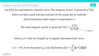
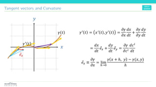
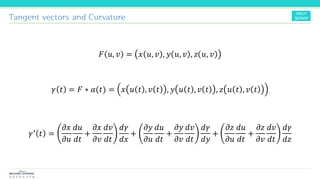
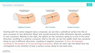
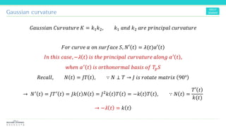
The document discusses the concepts and mathematical principles of manifold learning and interpolation in high dimensions, focusing on the properties of topological spaces and smooth manifolds. It elaborates on techniques such as parametric curves, tangent vectors, curvature, and geodesics, providing examples and deriving key equations related to these concepts. Additionally, it includes references for further reading on differential geometry and its applications.

2. Introduction
Introduction

3. Introduction
Interpolation in high dimension Interpolation in manifold

4. Learning on Manifolds
Learning 3D body shape on the sphere Learning Tree of Life on Poincaré disk

5. Basic Concepts
Basic Concepts

6. Topological Space
A topology on a set 𝑋 is a collection 𝜏 of subsets of 𝑋, satisfying the following axioms:
(1) The ∅ and 𝑋 itself are in 𝜏.
(2) The union of any collection of sets in 𝜏 is also in 𝜏
(3) The intersection of any finite number of sets in 𝜏 is also in 𝜏
𝑋 with its topology 𝜏 is called a topological space (𝑋, 𝜏).

7. Hausdorff Space

8. Topological Manifolds
Hausdorff, Second countable, paracompactness
-> metrizable space
(homeomorphic to a metric space – which means measurable space)
This means that, any points in the space 𝒳 × 𝒳 → ℝ+
Locally Euclidean

9. Smooth (differentiable) Manifolds
𝑝 𝑞
Totally different ℝ 𝑛
𝜑 𝛼 𝑝
𝑢 𝛼 𝑢 𝛽
𝜑 𝛼 𝑝 = (𝑥1
, 𝑥2
, ⋯, 𝑥 𝑛
)
N-tuple
𝜑 𝛼
−1 ∙ 𝜑 𝛼 𝑝 = 𝑝
𝜑 𝛽 ∙ 𝜑 𝛼
−1 𝑢 𝛼 = 𝑢 𝛽
If 𝜑 𝛽 ∙ 𝜑 𝛼
−1 is infinitely differentiable 𝐶∞, we call it
Smooth manifolds
Def: A smooth manifold or 𝐶∞ -manifold is a differentiable manifold for which all the transition maps are
smooth. That is, derivatives of all orders exist; so it is a 𝐶 𝑘 -manifold for all 𝑘. An equivalence class of such
atlases is said to be a smooth structure.

10. Diffeomorphism
𝑋
𝑌
𝑚𝑚
𝑓: 𝑋 → 𝑌
𝛾 ∙ 𝑓 ∙ 𝜑−1: 𝑅 𝑛 → 𝑅 𝑚
𝛾
If 𝛾 ∙ 𝑓 ∙ 𝜑−1 is infinitely differentiable 𝐶∞, 𝑓 is bijection, and 𝑓−1 is also differentiable,
then 𝑋 𝑎𝑛𝑑 𝑌 are diffeomorphic and 𝑓 is diffeomorphism

11. Specific Examples
Specific Examples

12. Specific Examples
Specific Examples

13. Parametric curves
In mathematics, a parametric equation defines a group of quantities as functions of one or more
independent variables called parameters. Parametric equations are commonly used to express the
coordinates of the points that make up a geometric object such as a curve or surface, in which case
the equations are collectively called a parametric representation or parameterization (alternatively
spelled as parametrisation) of the object.
For example, the equations
𝑥 = cos 𝑡
𝑦 = sin 𝑡
𝛾 𝑡 = 𝑥 𝑡 , 𝑦 𝑡 = (cos 𝑡 , sin 𝑡)
form a parametric representation of the unit circle, where t is the parameter: A point (𝑥, 𝑦) is on the
unit circle if and only if there is a value of t such that these two equations generate that point.

14. Parametric curves
We can also find other charts to map the unit
circle. Let's take a look at another construction
using standard Euclidean coordinates and a
stereographic projection. Figure 5 shows a
picture of this construction. We can define two
charts by taking either the "north" or "south"
pole of the circle, finding any other point on the
circle and projecting the line segment onto the
𝑥 − 𝑎𝑥𝑖𝑠 . This provides the mapping from a
point on the manifold to ℝ1. The "north" pole
point is visualized in blue, while the "south" pole
point is visualized in burgundy. Note: the local
coordinates for the charts are different. The
same point on the circle mapped via the two
charts do not map to the same point in ℝ1.
𝑢1: = 𝜑1(𝑝) =
𝜑1(𝑝)
1
=
𝑥 𝑝
1 − 𝑦𝑝

15. Specific Examples
Specific Examples

16. Tangent vectors and Curvature
𝐿𝑒𝑡 𝛾 𝑡 𝑏𝑒 𝑎 𝑝𝑎𝑟𝑎𝑚𝑒𝑡𝑟𝑖𝑐 𝑠𝑚𝑜𝑜𝑡ℎ 𝑐𝑢𝑟𝑣𝑒. 𝑇ℎ𝑒 𝑡𝑎𝑛𝑔𝑒𝑛𝑡 𝑣𝑒𝑐𝑡𝑜𝑟 𝑖𝑠 𝑔𝑖𝑣𝑒𝑛 𝑏𝑦 𝛾′ 𝑡 ,
𝑤ℎ𝑒𝑟𝑒 𝑤𝑒 ℎ𝑎𝑣𝑒 𝑢𝑠𝑒𝑑 𝑎 𝑝𝑟𝑖𝑚𝑒 𝑖𝑛𝑠𝑡𝑒𝑎𝑑 𝑜𝑓 𝑡ℎ𝑒 𝑢𝑠𝑢𝑎𝑙 𝑑𝑜𝑡 𝑡𝑜 𝑖𝑛𝑑𝑖𝑐𝑎𝑡𝑒
𝑑𝑖𝑓𝑓𝑒𝑟𝑒𝑛𝑡𝑖𝑎𝑡𝑖𝑜𝑛 𝑤𝑖𝑡ℎ 𝑟𝑒𝑠𝑝𝑒𝑐𝑡 𝑡𝑜 𝑝𝑎𝑟𝑎𝑚𝑒𝑡𝑒𝑟 𝑡.
𝑇ℎ𝑒 𝑢𝑛𝑖𝑡 𝑡𝑎𝑛𝑔𝑒𝑛𝑡 𝑣𝑒𝑐𝑡𝑜𝑟 𝑖𝑠 𝑔𝑖𝑣𝑒𝑛 𝑏𝑦 𝑇 𝑡 =
𝛾′
𝑡
𝛾′ 𝑡
𝐺𝑖𝑣𝑒𝑛 𝑡0 ∈ 𝐼, 𝑡ℎ𝑒 𝑎𝑟𝑐 𝑙𝑒𝑛𝑔𝑡ℎ 𝑜𝑓 𝑎 𝑟𝑒𝑔𝑢𝑙𝑎𝑟 𝑝𝑎𝑟𝑎𝑚𝑒𝑡𝑟𝑖𝑧𝑒𝑑 𝑐𝑢𝑟𝑣𝑒
𝛾: 𝐼 → 𝑅3, 𝑓𝑟𝑜𝑚 𝑡ℎ𝑒 𝑝𝑜𝑖𝑛𝑡 𝑡0, 𝑖𝑠 𝑏𝑦 𝑑𝑒𝑓𝑖𝑛𝑖𝑡𝑖𝑜𝑛 𝑠 𝑡 = න
𝑡0
𝑡
𝛾′ 𝑡 𝑑𝑡
speed

17. Tangent vectors and Curvature
𝛾′ 𝑡 = 𝑥′ 𝑡 , 𝑦′ 𝑡 =
𝜕𝛾
𝜕𝑥
𝑑𝑥
𝑑𝑡
+
𝜕𝛾
𝜕𝑦
𝑑𝑦
𝑑𝑡
=
𝑑𝑥
𝑑𝑡
Ԧ𝑒 𝑥 +
𝑑𝑦
𝑑𝑡
Ԧ𝑒 𝑦 =
𝜕𝛾
𝜕𝑐 𝑖
𝑑𝑐 𝑖
𝑑𝑡
Ԧ𝑒 𝑥 ≡
𝜕𝛾
𝜕𝑥
= lim
ℎ→0
𝛾 𝑥 + ℎ, 𝑦 − 𝛾(𝑥, 𝑦)
ℎ
𝛾′ 𝑡
𝛾 𝑡
Ԧ𝑒 𝑥

18. Tangent vectors and Curvature
𝐹 𝑢, 𝑣 = 𝑥 𝑢, 𝑣 , 𝑦 𝑢, 𝑣 , 𝑧 𝑢, 𝑣
𝛾 𝑡 = 𝐹 ∗ 𝛼(𝑡) = 𝑥 𝑢 𝑡 , 𝑣 𝑡 , 𝑦 𝑢 𝑡 , 𝑣 𝑡 , 𝑧 𝑢 𝑡 , 𝑣 𝑡
𝛾′ 𝑡 =
𝜕𝑥
𝜕𝑢
𝑑𝑢
𝑑𝑡
+
𝜕𝑥
𝜕𝑣
𝑑𝑣
𝑑𝑡
𝑑𝛾
𝑑𝑥
+
𝜕𝑦
𝜕𝑢
𝑑𝑢
𝑑𝑡
+
𝜕𝑦
𝜕𝑣
𝑑𝑣
𝑑𝑡
𝑑𝛾
𝑑𝑦
+
𝜕𝑧
𝜕𝑢
𝑑𝑢
𝑑𝑡
+
𝜕𝑧
𝜕𝑣
𝑑𝑣
𝑑𝑡
𝑑𝛾
𝑑𝑧

19. Tangent vectors and Curvature
𝐿𝑒𝑡 𝛼 ∶ 𝐼 𝑎, 𝑏 → 𝑅 𝑛 𝑏𝑒 𝑎 𝑝𝑎𝑟𝑎𝑚𝑒𝑡𝑟𝑖𝑠𝑒𝑑 𝑐𝑢𝑟𝑣𝑒, 𝑝𝑎𝑟𝑎𝑚𝑒𝑡𝑟𝑖𝑠𝑒𝑑 𝑏𝑦 𝑎𝑟𝑐 𝑙𝑒𝑛𝑔𝑡ℎ
𝑖. 𝑒 𝑛𝑜𝑟𝑚 𝑜𝑓 𝑡𝑎𝑛𝑔𝑒𝑛𝑡 𝑣𝑒𝑐𝑡𝑜𝑟 𝛼′ 𝑠 = 1 𝑓𝑜𝑟 𝑎𝑙𝑙 𝑠 .
𝑇ℎ𝑒 𝑐𝑢𝑟𝑣𝑎𝑡𝑢𝑟𝑒 𝑜𝑓 𝛼 𝑎𝑡 𝑡ℎ𝑒 𝑝𝑜𝑖𝑛𝑡 𝛼(𝑠) 𝑖𝑠 𝑡ℎ𝑒 𝑓𝑢𝑛𝑐𝑡𝑖𝑜𝑛
𝜅(𝑠) = ‖𝛼′′(𝑠)‖.
𝐼𝑡 𝑖𝑠 𝑡𝑟𝑎𝑑𝑖𝑡𝑖𝑜𝑛𝑎𝑙𝑙𝑦 𝑑𝑒𝑛𝑜𝑡𝑒𝑑 𝑏𝑦 𝑡ℎ𝑒 𝑔𝑟𝑒𝑒𝑘 𝑙𝑒𝑡𝑡𝑒𝑟 𝜅 𝑘𝑎𝑝𝑝𝑎
𝜅 𝑠 : a measure of how rapidly the curve pulls away from the tangent line at s

20. Tangent vectors and Curvature
𝛾 𝑠 = 𝑟(cos
𝑠
𝑟
,sin
𝑠
𝑟
)
𝛾′ 𝑠 = 𝑇 𝑠 = − sin
𝑠
𝑟
, cos
𝑠
𝑟
𝜅 𝑠 = 𝑇′ 𝑠 =
1
𝑟

21. Tangent vectors and Curvature
𝐿𝑒𝑡 𝛾′ 𝑠 ℎ𝑎𝑠 𝑎 𝑢𝑛𝑖𝑡 𝑙𝑒𝑛𝑔𝑡ℎ 𝑖. 𝑒 𝑛𝑜𝑟𝑚 𝑜𝑓 𝑡𝑎𝑛𝑔𝑒𝑛𝑡 𝑣𝑒𝑐𝑡𝑜𝑟 𝛾′ 𝑠 = 1 𝑓𝑜𝑟 𝑎𝑙𝑙 𝑠 .
𝐹𝑜𝑟 𝑇 𝑠 = 𝛾′ 𝑠 ,
𝑇 𝑠 ∙ 𝑇 𝑠 = 1
𝑇′ 𝑠 ∙ 𝑇 𝑠 = 0
⇒ 𝑇′ 𝑠 ⊥ 𝑇 𝑠
𝑎𝑛𝑑 𝑤𝑒 𝑑𝑒𝑓𝑖𝑛𝑒 𝑁 𝑠 =
𝛾′′ 𝑠
𝑘(𝑠)
𝑖𝑠 𝑛𝑜𝑟𝑚𝑎𝑙 𝑡𝑜 𝛾 𝑠 𝑎𝑛𝑑 𝑖𝑠 𝑐𝑎𝑙𝑙𝑒𝑑 𝑛𝑜𝑟𝑚𝑎𝑙 𝑣𝑒𝑐𝑡𝑜𝑟 𝑎𝑡 𝑠.

22. Specific Examples
Specific Examples

23. Tangent space and Normal vector
𝐴 𝑠𝑒𝑡 𝑜𝑓 𝑡𝑎𝑛𝑔𝑒𝑛𝑡 𝑣𝑒𝑐𝑡𝑜𝑟𝑠 𝑡𝑜 𝑚𝑎𝑛𝑖𝑓𝑜𝑙𝑑 𝑀 𝑎𝑡 𝑥 𝑖𝑠 𝑑𝑒𝑛𝑜𝑡𝑒𝑑 𝑏𝑦 𝑇𝑥 𝑀

24. Tangent space and Normal vector
𝐿𝑒𝑡 𝛽: −𝜖, 𝜖 → 𝑈 ⊂ ℝ2, 𝛽 𝑡 = (𝑢 𝑡 , 𝑣 𝑡 )
𝑡ℎ𝑒𝑛, 𝑐𝑢𝑟𝑣𝑒 𝛼 𝑜𝑛 𝑠𝑢𝑟𝑓𝑎𝑐𝑒 𝑆 𝑖𝑠 𝑓𝑜𝑟𝑚𝑢𝑙𝑎𝑡𝑒𝑑 𝑎𝑠 𝑏𝑒𝑙𝑜𝑤:
𝛼 𝑡 = 𝑥 ∗ 𝛽 𝑡 = 𝑥 𝑢 𝑡 , 𝑣 𝑡
𝑡𝑎𝑛𝑔𝑒𝑛𝑡 𝑣𝑒𝑐𝑡𝑜𝑟 𝛼′(𝑡) =
𝜕𝑥
𝜕𝑢
𝑑𝑢
𝑑𝑡
+
𝜕𝑥
𝜕𝑣
𝑑𝑣
𝑑𝑡
= 𝒙 𝑢 𝑢′ 𝑡 + 𝒙 𝑣 𝑣′ 𝑡
𝑇ℎ𝑢𝑠, 𝒙 𝑢, 𝒙 𝑣 𝑎𝑟𝑒 𝑏𝑎𝑠𝑖𝑠 𝑜𝑓 𝑇𝑝 𝑆
𝑡
ℝ2
𝛽
𝑥
𝑆
𝛼

25. Tangent space and Normal vector
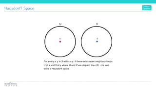
𝜎 𝑡
≝ 𝛾−1[ 𝛾 ∗ 𝜓 𝑡 + 𝑡0 + 𝛾 ∗ 𝜙 𝑡 + 𝑡1
− (𝛾 ∗ 𝜓)(𝑡0)]
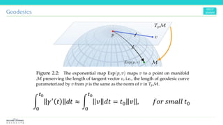
p
𝑡
𝑡0 𝑡1 𝑡2
ψ 𝜙 𝜎
𝛾 ℝ 𝑛
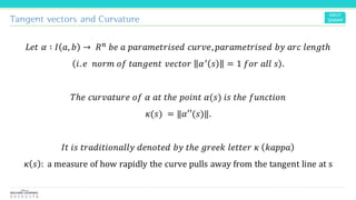
𝑝 = ψ 𝑡0 = 𝜙(𝑡1) = 𝜎 𝑡2
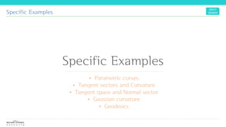
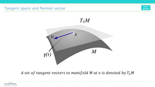
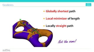
𝑇ℎ𝑒𝑟𝑒 𝑒𝑥𝑖𝑠𝑡 𝑎 𝑐𝑢𝑟𝑣𝑒 𝜎, 𝑎𝑛𝑑 𝑤𝑒 𝑐𝑎𝑛 𝑎𝑐𝑡𝑢𝑎𝑙𝑙𝑦
𝑐𝑜𝑛𝑠𝑡𝑟𝑢𝑐𝑡 𝑡ℎ𝑎𝑡 𝑤𝑖𝑙𝑙 𝑟𝑒𝑝𝑟𝑒𝑠𝑒𝑛𝑡 𝑠𝑢𝑚 𝑜𝑓 𝑡𝑤𝑜 𝑐𝑢𝑟𝑣𝑒𝑠
𝒱𝑝,ψ + 𝒱𝑝,𝜙 = 𝒱𝑝,𝜎
𝐼𝑡 𝑠ℎ𝑜𝑤𝑠 𝑦𝑜𝑢 ℎ𝑜𝑤 𝑤𝑒 𝑎𝑟𝑒 𝑔𝑜𝑖𝑛𝑔 𝑡𝑜 𝑐𝑜𝑛𝑠𝑡𝑟𝑢𝑐𝑡
𝑣𝑒𝑐𝑡𝑜𝑟 𝑠𝑝𝑎𝑐𝑒 ( 𝑇𝑝 𝑀) 𝑏𝑦 𝑡𝑎𝑛𝑔𝑒𝑛𝑡 𝑣𝑒𝑐𝑡𝑜𝑟
𝑓 ∈ 𝐶∞
ℝ

26. Tangent space and Normal vector
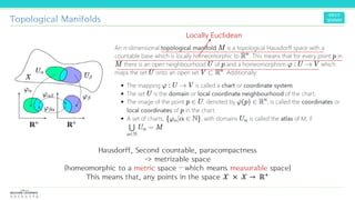
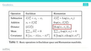
p
𝑡
𝑡0 𝑡1 𝑡2
ψ 𝜙 𝜎
𝛾 ℝ 𝑛
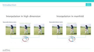
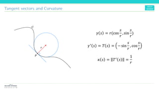
𝑝 = ψ 𝑡0 = 𝜙(𝑡1) = 𝜎 𝑡2
ℝ 𝑀 ℝ
ℝ 𝑛
𝜎 𝑓
𝛾 ∗ 𝜎 𝑓 ∗ 𝛾−1
𝛾
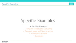
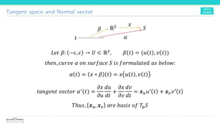
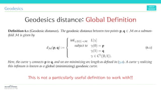
𝐿𝑒𝑡 𝑡2 = 0 𝑡ℎ𝑒𝑛,
𝜎 0 = 𝛾−1[ 𝛾 ∗ 𝜓 𝑡0 + 𝛾 ∗ 𝜙 𝑡1
−(𝛾 ∗ 𝜓)(𝑡0)]
= 𝑝
𝑓 ∈ 𝐶∞
ℝ

27. Tangent space and Normal vector
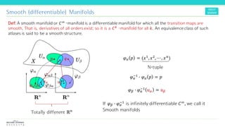
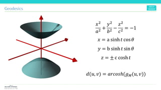
ℝ 𝑀 ℝ
ℝ 𝑛
𝜎 𝑓
𝛾 ∗ 𝜎 𝑓 ∗ 𝛾−1
𝛾
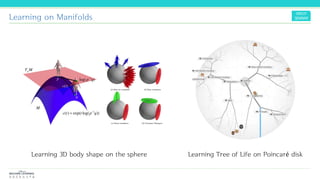
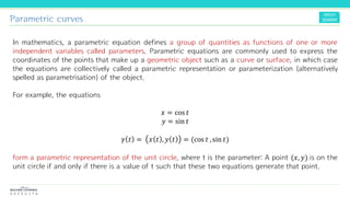
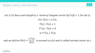
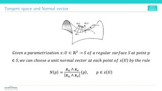
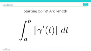
𝒱𝑝,𝜎 𝑓 = (𝑓 ∗ 𝜎)′(0) = 𝒱𝑝,ψ 𝑓 + 𝒱𝑝,𝜙 𝑓
𝒱𝑝,𝜎 𝑓 = (𝑓 ∗ 𝜎)′(0) = (𝑓 ∗ 𝛾−1 ∗ 𝛾 ∗ 𝜎)′(0) = { 𝑓 ∗ 𝛾−1 ∗ 𝛾 ∗ 𝜎 }′(0)
=
𝜕𝑗 𝑓 ∗ 𝛾−1 𝛾 ∗ 𝜎
𝜕(𝛾 ∗ 𝜎) 𝑗
𝑑(𝛾 ∗ 𝜎) 𝑗
𝑑𝑡
[0]
𝑓

28. Tangent space and Normal vector
ℝ 𝑀 ℝ
ℝ 𝑛
𝜎 𝑓
𝛾 ∗ 𝜎 𝑓 ∗ 𝛾−1
𝛾
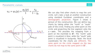
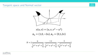
𝑑(𝛾 ∗ 𝜎) 𝑗
𝑑𝑡
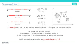
[0] = (𝛾 ∗ 𝜎) 𝑗′
0 = {𝛾 ∗ 𝛾−1 ∗ 𝛾 ∗ 𝜓 𝑡 + 𝑡0 + 𝛾 ∗ 𝛾−1 ∗ 𝛾 ∗ 𝜙 𝑡 + 𝑡0
−𝛾 ∗ 𝛾−1 ∗ 𝛾 ∗ 𝜓 𝑡0 } 𝑗′
0
= (𝛾 ∗ 𝜓) 𝑗′
𝑡0 + (𝛾 ∗ 𝜙) 𝑗′
𝑡1 = 𝒱𝑝,ψ + 𝒱𝑝,𝜙
This is not a function of 𝑡

29. Tangent space and Normal vector
𝐺𝑖𝑣𝑒𝑛 𝑎 𝑝𝑎𝑟𝑎𝑚𝑒𝑡𝑟𝑖𝑧𝑎𝑡𝑖𝑜𝑛 𝑥: 𝑈 ⊂ ℝ2 → 𝑆 𝑜𝑓 𝑎 𝑟𝑒𝑔𝑢𝑙𝑎𝑟 𝑠𝑢𝑟𝑓𝑎𝑐𝑒 𝑆 𝑎𝑡 𝑝𝑜𝑖𝑛𝑡 𝑝
∈ 𝑆, 𝑤𝑒 𝑐𝑎𝑛 𝑐ℎ𝑜𝑜𝑠𝑒 𝑎 𝑢𝑛𝑖𝑡 𝑛𝑜𝑟𝑚𝑎𝑙 𝑣𝑒𝑐𝑡𝑜𝑟 𝑎𝑡 𝑒𝑎𝑐ℎ 𝑝𝑜𝑖𝑛𝑡 𝑜𝑓 𝑥 𝑈 𝑏𝑦 𝑡ℎ𝑒 𝑟𝑢𝑙𝑒
𝑁 𝑝 =
𝒙 𝑢 ∧ 𝒙 𝑣
𝒙 𝑢 ∧ 𝒙 𝑣
𝑝 , 𝑝 ∈ 𝑥 𝑈

30. Tangent space and Normal vector
𝑥 𝑢, 𝑣 = 𝑢, 𝑣, 𝑣2 − 𝑢2
𝒙 𝑢 = 1,0, −2𝑢 , 𝒙 𝑣 = 0,1,2𝑣
𝑁 = (
𝑢
𝑣2 + 𝑢2 +
1
4
,
−𝑣
𝑣2 + 𝑢2 +
1
4
,
1
2 𝑣2 + 𝑢2 +
1
4
)

31. Specific Examples
Specific Examples

32. Gaussian curvature
Starting with the center diagram (zero curvature), we see that a cylindrical surface has flat or
zero curvature in one dimension (blue) and curved around the other dimension (green), resulting
in zero curvature. Moving to the right, the sphere on has curvature along its to axis in the same
direction, resulting in a positive curvature. And to the left, we see the saddle sheet has curvature
along its axis in different directions, resulting in negative curvature. In fact, the Gaussian
curvature is the product of its two principal curvatures, which we won't get into detail here but
corresponds to our intuition of how a surface curves along its two main axes.

33. Gaussian curvature
𝐺𝑎𝑢𝑠𝑠𝑖𝑎𝑛 𝐶𝑢𝑟𝑣𝑎𝑡𝑢𝑟𝑒 𝐾 = 𝑘1 𝑘2, 𝑘1 𝑎𝑛𝑑 𝑘2 𝑎𝑟𝑒 𝑝𝑟𝑖𝑛𝑐𝑖𝑝𝑎𝑙 𝑐𝑢𝑟𝑣𝑎𝑡𝑢𝑟𝑒
𝐹𝑜𝑟 𝑐𝑢𝑟𝑣𝑒 𝛼 𝑜𝑛 𝑠𝑢𝑟𝑓𝑎𝑐𝑒 𝑆, 𝑁′ 𝑡 = 𝜆(𝑡)𝛼′ 𝑡
𝐼𝑛 𝑡ℎ𝑖𝑠 𝑐𝑎𝑠𝑒,−𝜆 𝑡 𝑖𝑠 𝑡ℎ𝑒 𝑝𝑟𝑖𝑛𝑐𝑖𝑝𝑎𝑙 𝑐𝑢𝑟𝑣𝑎𝑡𝑢𝑟𝑒 𝑎𝑙𝑜𝑛𝑔 𝛼′
𝑡 ,
𝑤ℎ𝑒𝑛 𝛼′
𝑡 𝑖𝑠 𝑜𝑟𝑡ℎ𝑜𝑛𝑜𝑟𝑚𝑎𝑙 𝑏𝑎𝑠𝑖𝑠 𝑜𝑓 𝑇𝑝 𝑆
𝑅𝑒𝑐𝑎𝑙𝑙, 𝑁 𝑡 = 𝐽𝑇 𝑡 , ∵ 𝑁 ⊥ 𝑇 → 𝐽 𝑖𝑠 𝑟𝑜𝑡𝑎𝑡𝑒 𝑚𝑎𝑡𝑟𝑖𝑥 90°
→ 𝑁′
𝑡 = 𝐽𝑇′
𝑡 = 𝐽𝑘 𝑡 𝑁 𝑡 = 𝐽2
𝑘 𝑡 𝑇 𝑡 = −𝑘 𝑡 𝑇 𝑡 , ∵ 𝑁 𝑡 =
𝑇′ 𝑡
𝑘(𝑡)
→ −𝜆 𝑡 = 𝑘 𝑡

34. Specific Examples
Specific Examples

35. Geodesics

36. Geodesics
Geodesics distance: Global Definition
This is not a particularly useful definition to work with!!

37. Geodesics
Starting point: Arc length

38. Geodesics
𝐴 𝑐𝑢𝑟𝑣𝑒 𝛾 s,t will be function of two real parameter,
t is time and s is variation of curve
if we fix s,then only t is chaging,
we give it another notation 𝛾𝑠 t , 𝑡ℎ𝑖𝑠 𝑖𝑠 𝑓𝑢𝑛𝑐𝑡𝑖𝑜𝑛 𝑜𝑓 𝑡
we call it 𝑔𝑒𝑜𝑑𝑒𝑠𝑖𝑐𝑠 if
𝑑
𝑑𝑠
ㅣ 𝑠=0 𝐿 𝛾𝑠 = 0
𝐴 𝑓𝑎𝑚𝑖𝑙𝑙𝑦 𝑜𝑓 𝛾𝑠
𝛾(𝑎) 𝛾(𝑏)
𝛾𝑠=𝑐(𝑘)
𝛾𝑠=𝑑(𝑘)
𝛾0(𝑘)
𝑇ℎ𝑒 𝑑𝑜𝑡𝑡𝑒𝑑 𝑐𝑢𝑟𝑣𝑒 𝑖𝑠 𝑠(−𝜀, 𝜀) → 𝛾𝑠 𝑡
𝑑
𝑑𝑠
𝛾𝑠 𝑘 𝑎𝑛𝑑
𝑑
𝑑𝑡
𝛾0 𝑡 𝑎𝑟𝑒 𝑖𝑛 𝑇𝛾 𝑠 𝑡
𝑤ℎ𝑒𝑛 𝑠 = 0, 𝑡 = 𝑘
𝑠 = 0
𝑡 = 𝑘

39. Geodesics

40. Geodesics
𝑑
𝑑𝑠
𝐿 𝛾𝑠 =
𝑑
𝑑𝑠
1
2
න
𝑎
𝑏
𝛾′ 𝑠(𝑡) 2 𝑑𝑡 = න
𝑎
𝑏
𝑑
𝑑𝑠
< 𝛾′ 𝑠(𝑡), 𝛾′ 𝑠(𝑡) > 𝑑𝑡
= න
𝑎
𝑏
<
𝑑𝛾′ 𝑠(𝑡)
𝑑𝑠
, 𝛾′ 𝑠(𝑡) > 𝑑𝑡 = <
𝑑𝛾𝑠 𝑡
𝑑𝑠
, 𝛾′
𝑠 𝑡 > − න
𝑎
𝑏
<
𝑑𝛾𝑠(𝑡)
𝑑𝑠
, 𝛾′′ 𝑠(𝑡) > 𝑑𝑡
𝐼𝑚𝑝𝑜𝑟𝑡𝑎𝑛𝑡 𝑝𝑜𝑖𝑛𝑡 𝑖𝑠 𝑡ℎ𝑎𝑡 𝛾 𝑠, 𝑎 and 𝛾 𝑠, 𝑏 𝑎𝑟𝑒 𝑓𝑖𝑥𝑒𝑑 𝑓𝑜𝑟 𝑎𝑙𝑙 𝑠
→
𝑑𝛾𝑠 𝑎
𝑑𝑠
=
𝑑𝛾𝑠 𝑏
𝑑𝑠
= 0

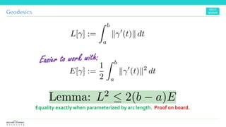
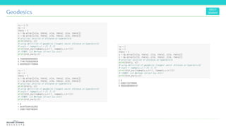
41. Geodesics
න
𝑎
𝑏
<
𝑑𝛾′ 𝑠(𝑡)
𝑑𝑠
, 𝛾′ 𝑠(𝑡) > 𝑑𝑡 = <
𝑑𝛾𝑠 𝑡
𝑑𝑠
, 𝛾′
𝑠 𝑡 > − න
𝑎
𝑏
<
𝑑𝛾𝑠 𝑡
𝑑𝑠
, 𝛾′′
𝑠 𝑡 > 𝑑𝑡
= − න
𝑎
𝑏
<
𝑑𝛾𝑠 𝑡
𝑑𝑠
, 𝛾′′
𝑠 𝑡 > 𝑑𝑡 = − න
𝑎
𝑏
<
𝑑𝛾𝑠 𝑡
𝑑𝑠
, 𝑃𝑟𝑜𝑗 𝑇 𝛾 𝑠 𝑡
𝛾′′
𝑠 𝑡 > 𝑑𝑡 = 0
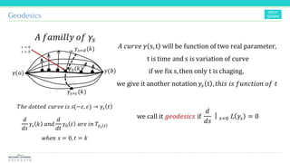
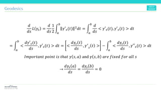
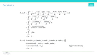
𝑇ℎ𝑖𝑠 𝑖𝑚𝑙𝑖𝑒𝑠 𝑡ℎ𝑎𝑡 𝑖𝑓 𝑎 𝑐𝑢𝑟𝑣𝑒 𝛾: 𝑎, 𝑏 → 𝑀 𝑖𝑠 𝑎 𝑔𝑒𝑜𝑑𝑒𝑠𝑖𝑐, 𝑡ℎ𝑒𝑛
𝑃𝑟𝑜𝑗 𝑇 𝛾 𝑠 𝑡
𝛾′′
𝑠 𝑡 = 0
𝑓𝑜𝑟 𝑡 ∈ [𝑎, 𝑏]
= 0
Note that it is in 𝑇𝛾𝑠 𝑡

42. 𝐼𝑛𝑡𝑢𝑡𝑖𝑜𝑛 𝑜𝑓 𝑃𝑟𝑜𝑗 𝑇 𝛾 𝑠 𝑡
𝛾′′
𝑠 𝑡 ≡ 0
Geodesics

43. Geodesics

44. Geodesics
න
0
𝑡0
𝛾′
𝑡 𝑑𝑡 ≈ න
0
𝑡0
𝑣 𝑑𝑡 = 𝑡0 𝑣 , 𝑓𝑜𝑟 𝑠𝑚𝑎𝑙𝑙 𝑡0

45. Geodesics

46. Geodesics
𝑥2
𝑎2
+
𝑦2
𝑏2
−
𝑧2
𝑐2
= −1
𝑥 = a sinh 𝑡 cos 𝜃
𝑦 = b sinh 𝑡 sin 𝜃
𝑧 = ± c cosh 𝑡
𝑑(𝑢, 𝑣) = 𝑎𝑟𝑐𝑜𝑠ℎ(𝑔 𝑀(𝑢, 𝑣))

47. Geodesics

48. Geodesics

49. Geodesics

50. References
References

51. References
Differential Geometry of Curves and Surfaces, Manfredo P. Do Carmo (2016)
Differential Geometry by Claudio Arezzo
Youtube: https://youtu.be/tKnBj7B2PSg
What is a Manifold?
Youtube: https://youtu.be/CEXSSz0gZI4
Shape analysis (MIT spring 2019) by Justin Solomon
Youtube: https://youtu.be/GEljqHZb30c
Tensor Calculus
Youtube: https://youtu.be/kGXr1SF3WmA
Manifolds: A Gentle Introduction,
Hyperbolic Geometry and Poincaré Embeddings by Brian Keng
Link: http://bjlkeng.github.io/posts/manifolds/,
http://bjlkeng.github.io/posts/hyperbolic-geometry-and-poincare-embeddings/
Statistical Learning models for Manifold-Valued measurements with application to computer vision and
neuroimaging by Hyunwoo J.Kim