Download as PDF, PPTX

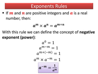
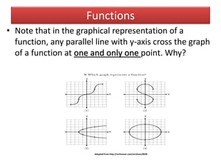
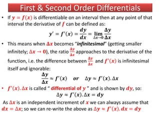
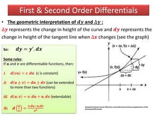
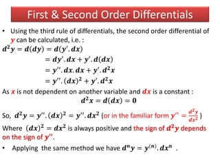
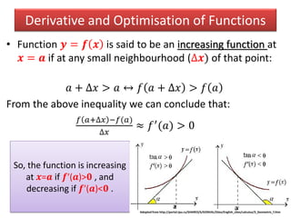
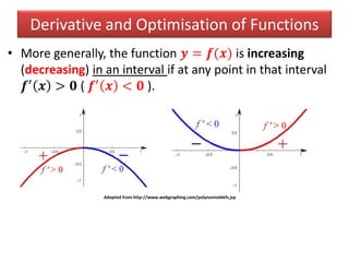
![Inflection Point & Concavity of Function
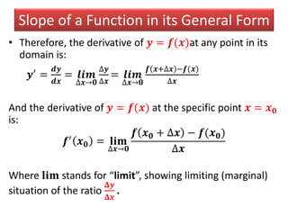
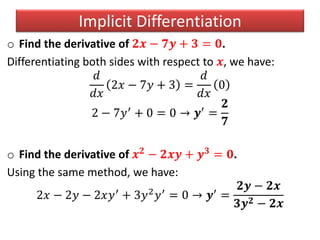
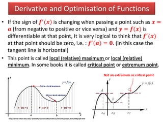
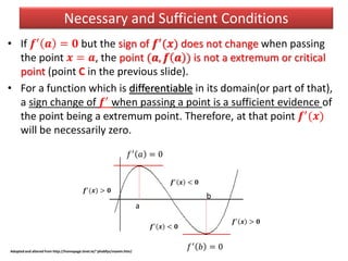
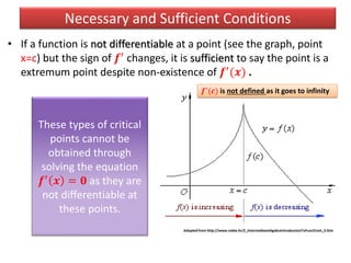
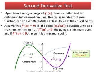
• If 𝒇′ 𝒂 = 𝟎 and at the same time 𝒇′′ 𝒂 = 𝟎, we need other tests
to find out the nature of the point. It could be a extremum point
[e.g. 𝒚 = 𝒙 𝟒
, which has minimum at 𝒙 = 𝟎]or just an inflection
point (where the tangent line crosses the graph of the function and
separate that to two parts; concave up and concave down)
Adopted and altered from http://www.ltcconline.net/greenl/courses/105/curvesketching/SECTST.HTM Adopted from http://www.sparkle.pro.br/tutorial/geometry
𝑓′′ 𝑥 = 0
𝑓′ 𝑥 > 0
Concave Down
Concave up](https://image.slidesharecdn.com/basiccalculusi-150114142144-conversion-gate01/85/Basic-calculus-i-52-320.jpg)

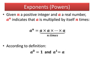
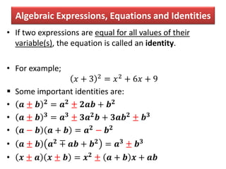
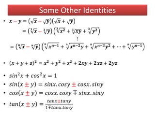
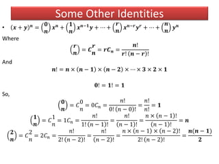
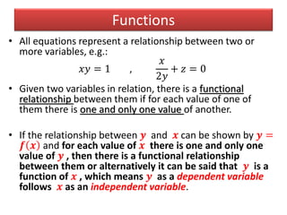
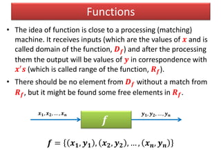
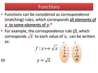
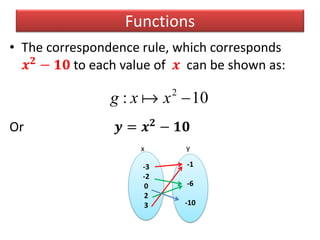
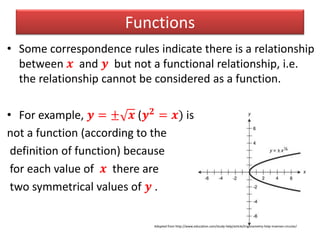
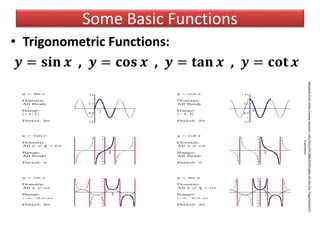
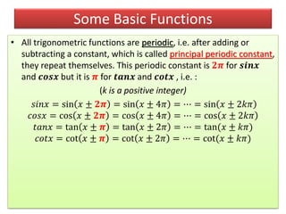
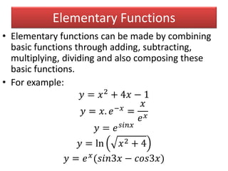
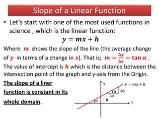
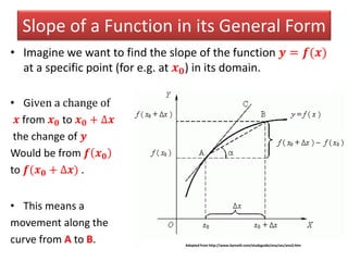
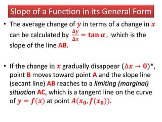
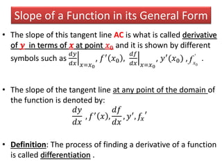
The document provides an overview of basic calculus concepts including: - Exponents and exponent rules for multiplying, dividing, and raising to powers. - Algebraic expressions including monomials, binomials, polynomials, and equations. - Common identities for exponents, polynomials, trigonometric functions. - The definition of a function as a correspondence between variables where each input has a single output. - Examples of basic functions including power, exponential, logarithmic, and trigonometric functions.