Materials Engineering Lecture Notes

1
BME 205
Materials Engineering (M)
B. Tech, 4th Semester
Veer Surendra Sai University of Technology, Burla, Sambalpur, Odisha
Course Coordinator
1. Renu Kumari
Assistant Professor
Department of Metallurgical & Materials Engineering (MME)
Email: renumetalbit@gmail.com, Mob. No-09564452009
2. Suneeti Purohit
Assistant Professor
E-mail: suneeti.purohit@gmail.com Mob. No: (+91) 8339037187
3. Gautam Behera
Assistant Professor
Email: gautamiitkgpian@gmail.com, Mob. No: +91 7855856611

2
Module-1
Introduction of Materials Science and Engineering
Materials Science – Investigating relationships that exist between the structure and properties of
materials.
Materials Engineering – On the basis of these structure-property correlations, designing or
engineering the structure of a material to produce a pre-determined set of properties.
Structure
Structure of a material usually relates to the arrangement of its internal components.
 Subatomic - Structure involves electrons within the individual atoms and interactions with
their nuclei.
 Atomic level- structure encompasses the organization of atoms or molecules relative to one
another.
 Microscopic – Which contains large groups of atoms that are normally agglomerated
together.
 Macroscopic – Viewable with the naked eye.
Property
A property is a material trait in terms of the kind and magnitude of response to a specific
imposed stimulus. Properties are made independent of material shape and size.
Example-
 A specimen subjected to forces will experience deformation,
 A polished metal surface will reflect light.
Properties of solid materials may be grouped into six different categories: (1) mechanical,
(2) electrical, (3) thermal, (4) magnetic, (5) optical and (6) deteriorative. The four components of
the discipline of materials science and engineering and their interrelationship.

3
Classification of Materials
Solid materials have been conveniently grouped into three basic classifications:
(1) metals, (2) ceramics, and (3) polymers.
Metals
 Materials in this group are composed of one or more metallic elements (such as iron,
aluminum, copper, titanium, gold, and nickel), and often also nonmetallic elements (for
example, carbon, nitrogen, and oxygen) in relatively small amounts.
 Atoms in metals and their alloys are arranged in a very orderly manner.
 In comparison to the ceramics and polymers, are relatively dense.
 Mechanical Property- relatively stiff and strong , ductile (i.e., capable of large amounts
of deformation without fracture), and are resistant to fracture.
 Metallic materials have large numbers of nonlocalized electrons; that is, these electrons
are not bound to particular atoms.Many properties of metals are directly attributable to
these electrons.
 Example, metals are extremely good conductors of electricity,and heat, and are not
transparent to visible light; a polished metal surface has a lustrous appearance.
 Some of the metals (viz., Fe, Co, and Ni) have desirable magnetic properties.
Ceramics
 Ceramics are compounds between metallic and nonmetallic elements; they are most
frequently oxides, nitrides, and carbides.
 Examples-aluminum oxide (or alumina, Al2O3), silicon dioxide (or silica, SiO2),silicon
carbide (SiC), silicon nitride (Si3N4).
 Examples of traditional ceramics — clay minerals (i.e., porcelain), cement, and glass.
Properties-
 Relatively stiff and strong—stiffnesses and strengths are comparable to those of the
metals , very hard, extremely brittle (lack ductility),.highly susceptible to fracture.
 Thermal and electrical Properties- Insulative to the passage of heat and electricity low
electrical conductivities and are more resistant to high temperatures
 Optical characteristics-Ceramics may be transparent, translucent, or opaque.

4
Polymers
 Carbon-based compounds.
 Chain of H-C molecules. Each repeat unit of H-C is a monomer e.g. ethylene (C2H4),
Polyethylene – (–CH2 –CH2)n.
 Polymers include the familiar plastic and rubber materials.
 Many of them are organic compounds that are chemically based on carbon, hydrogen,
and other nonmetallic elements (viz. O, N, and Si).
 They have very large molecular structures, often chain-like in nature that have a
backbone of carbon atoms. Some of the common and familiar polymers are polyethylene
(PE), nylon, poly (vinyl chloride)(PVC), polycarbonate (PC), polystyrene (PS), and
silicone rubber.
Properties
 Low densities, not as stiff nor as strong as ceramics and metals.
 Extremely ductile and pliable (i.e., plastic).
 Relatively inert chemically and unreactive in a large number of environments.
Limitations
 Tendency to soften and/or decompose at modest temperatures, which, in some
instances,limits their use.
 Low electrical conductivities and are nonmagnetic.
Composites
 A composite is composed of two (or more) individual materials, which come from the
categories discussed above—viz., metals, ceramics, and polymers.
 Objective-to achieve a combination of properties that is not displayed by any single
material
Examples
 Cemented carbides (WC with Co binder)
 Plastic molding compounds containing fillers
 Rubber mixed with carbon black

5
 Wood (a natural composite as distinguished from a synthesized composite)
Advance Materials
 Materials that are utilized in high-technology (or high-tech) applications are sometimes
termed advanced materials.
Examples
 Include electronic equipment (camcorders, CD/DVD players, etc.), computers, fiber-optic
systems, spacecraft, aircraft, and military rocketry, liquid crystal displays (LCDs), and
fiber optics.
 These advanced materials may be typically traditional materials types (e.g., metals,
ceramics, polymers) whose properties have been enhanced, and, also newly developed,
high-performance materials.
 Advanced materials include semiconductors, biomaterials, and what we may term“
materials of the future.
Biomaterials
 Biomaterials are employed in components implanted into the human body for
replacement of diseased or damaged body parts.
 These materials must not produce toxic substances and must be compatible with body
tissues (i.e., must not cause adverse biological reactions).
 All of the above materials—metals, ceramics, polymers, composites, and
semiconductors—may be used as biomaterials.
Example-
Titanium and its alloy, Co-Cr alloy, stainless steel, zirconia, HA, TiO2 etc.
Semiconductors
 Semiconductors have electrical properties that are intermediate between the electrical
conductors (viz. metals and metal alloys) and insulators (viz. ceramics and polymers).
 The electrical characteristics of these materials are extremely sensitive to the presence of
minute concentrations of impurity atoms, for which the concentrations may be controlled
over very small spatial regions.

6
 Semiconductors have made possible the advent of integrated circuitry that has totally
revolutionized the electronics and computer industries (not to mention our lives) over the
past three decades.
The Materials Selection Process
 Pick Application and determine required Properties.
 Properties: mechanical, electrical, thermal, magnetic, optical, deteriorative.
 Properties- Identify candidate Material(s)
 Material: structure, composition.
 Material- Identify required Processing
 Processing: changes structure and overall shape
Example: casting, sintering, vapor deposition, doping forming, joining, annealing.
Elastic deformation in metals:
 Deformation in which stress and strain are proportional is called elastic deformation.
 In elastic deformation a limited distortion of the crystal lattice is produced, but the atoms do
not move permanently from their ordered positions, and as soon as the stress is removed the
distortion disappears and the body returns to its original configuration (shape and size).
 When metal is stressed beyond the elastic limit plastic deformation takes place and there
must, clearly, be some movement of the atoms in to new positions, since considerable
permanent distortion can be produced.
 Usually in metals and ceramics elastic deformation is seen at low strains (< 10–3).
 Elasticity can be linear or Non linear. Metals and ceramics usually show linear elastic
behavior.
 Some materials (e.g., gray cast iron, concrete, and many polymers) exhibit non linear
elasticity.
F

bonds
stretch
return to
initial
Stress-Strain curve showing
linear elastic behavior

7
Plastic deformation in metals:
 Plastic deformation in the broadest sense means permanent deformation in the absence of
external constraints (forces, displacements).
 From an atomic perspective, plastic deformation corresponds to the breaking of bonds with
original atom neighbors and then reforming bonds with new neighbors as large numbers of
atoms or molecules move relative to one another; upon removal of the stress they do not
return to their original positions.
 For most metallic materials, elastic deformation persists only to strains of about 0.005. As
the material is deformed beyond this point, the stress is no longer proportional to strain
(Hooke’s law) and permanent/nonrecoverable/plastic deformation occurs.
 The transition from elastic to plastic is a gradual one for most metals; some curvature results
at the onset of plastic deformation, which increases more rapidly with rising stress..
 The mechanism of plastic deformation is not the same for all classes of materials and it is
necessary to consider the various materials groups separately.
 Metals, in general, are characterized by possessing high elastic modulus values, and also the
ability to be strained m a plastic manner.
Stress-Strain curve showing non-linear
elastic behavior

8
 Some metals will begin to deform plastically at very low values of stress and will yield to a
very considerable extent before fracture occurs. Other metals and alloys show little plastic
yielding before fracture. These latter materials are termed brittle.
Mechanism/Modes of plastic deformation in metals:
 Plastic deformation in crystalline solid is accomplished by means of various processes
mentioned below; among which slip is the most important mechanism.
 Plastic deformation of crystalline materials takes place by mechanisms which are very
different from that for amorphous materials (glasses).
 Plastic deformation in amorphous materials occurs by other mechanisms including flow
(~viscous fluid) and shear banding.

9
Plastic deformation by Slip:
 Slip is the most important mechanism of plastic deformation. At low temperatures
(especially in BCC metals) twinning may also become important.
 At the fundamental level plastic deformation (in crystalline materials) by slip involves the
motion of dislocations on the slip plane (creating a step of Burgers vector).
 Slip is caused by shear stresses (at the level of the slip plane). Hence, a purely hydrostatic
state of stress cannot cause slip.
 A slip system consists of a slip direction lying on a slip plane.
 Slip is analogous to the mode of locomotion employed by a caterpillar.

10
Microscopic slip to macroscopic deformation

11
Slip systems:
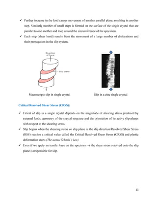
 Dislocations move more easily on specific planes and in specific directions.
 Ordinarily, there is a preferred plane (slip plane), and specific directions (slip direction)
along which dislocations move. The combination of slip plane and slip direction is called
the slip system.
 The slip system depends on the crystal structure of the metal.
 The slip plane is the plane that has the most dense atomic packing (the greatest planar
density). The slip direction is most closely packed with atoms (highest linear density)
Crystal Slip plane(s)
Slip direction
(b vector)
Number of
slip systems
FCC {111} ½<110> 12
HCP (0001) <1120> 3
BCC
{110}, {112},
{123}
½[111] 48
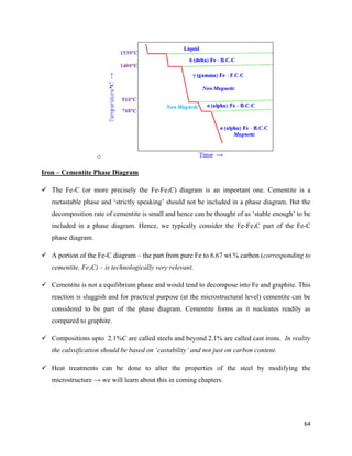
Stress to move a dislocation: Peierls – Nabarro (PN) stress:
 At the fundamental level the motion of a dislocation involves the rearrangement of bonds
which requires application of shear stress on the slip plane.
 Consider plastic deformation is the transition between unslipped to slipped state. As this
process is opposed by an energy barrier ΔE, the materials cannot make the transition
simultaneously.
 To minimize the energetic of the process the slipped material will grow at the expenses of
the unslipped region by the advance of an interfacial region (width of the dislocation w).

12
 The original model is due to Peierls & Nabarro (formula as below) and the ‘sufficient’ stress
which needs to be applied is called Peierls-Nabarro stress (PN stress) or simply Peierls
stress.
 Width of the dislocation is considered as a basis for the ease of motion of a dislocation in
the model which is a function of the bonding in the material.
 Peierls equation shows that wide dislocations will require low stress to move the
dislocations.
 In ceramics the interfacial energy is high and the dislocation width is very narrow. Hence
they are relatively immobile compared to ductile materials (dislocation width nearly 10
atomic spacings).
 Ceramics become ductile at high temperature as thermal activation help the dislocations to
overcome the energy barrier.
Slip in single crystal:
 If a single crystal of a metal is stressed in tension beyond its elastic limit, it elongates
slightly and a step appears on the surface due to the relative displacement of one part of the
crystal with respect to the others and the elongation stops.

13
 Further increase in the load causes movement of another parallel plane, resulting in another
step. Similarly number of small steps is formed on the surface of the single crystal that are
parallel to one another and loop around the circumference of the specimen.
 Each step (shear band) results from the movement of a large number of dislocations and
their propagation in the slip system.
Macroscopic slip in single crystal Slip in a zinc single crystal
Critical Resolved Shear Stress (CRSS):
 Extent of slip in a single crystal depends on the magnitude of shearing stress produced by
external loads, geometry of the crystal structure and the orientation of he active slip planes
with respect to the shearing stress.
 Slip begins when the shearing stress on slip plane in the slip direction/Resolved Shear Stress
(RSS) reaches a critical value called the Critical Resolved Shear Stress (CRSS) and plastic
deformation starts (The actual Schmid’s law)
 Even if we apply an tensile force on the specimen  the shear stress resolved onto the slip
plane is responsible for slip.

14







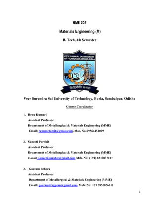
Area
Force
Stress










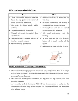
CosA
CosF
/
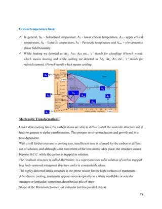
 CosCosRSS 
CosCos Schmid factor
 τ RSS is maximum (F/2A) when ϕ = λ=45o
 If the tension axis is normal to slip plane i.e. λ=90o
or if it is parallel to the slip plane i.e.
ϕ = 90o
then τ RSS = 0 and slip will not occur as per Schmid’s law.
 Schmid’s law: Slip is initiated when
 CRSS is a material parameter, which is determined from experiments
 Yield strength of a single crystal
Solved Example: Determine the tensile stress that is applied along the ]011[

axis of a silver
crystal to cause slip on the ]110)[111(

system. The critical resolved shear stress is 6 MPa.
Solution: ]Determine the angle ϕ between the tensile axis and normal to using the
following equation.
RSS CRSS 
CRSS
y
Cos Cos


 

]011[

)111(


15











))((
θcos 2
2
2
2
2
2
2
1
2
1
2
1
212121
wvuwvu
wwvvuu
6
2
32
1
])1()1()1][()0()1()1[(
)1)(0()1)(1()1)(1(
cos 222222












Determine the angle λ between tensile axis ]011[

and slip direction ]110[

2
1
22
1
])1()1()0][()0()1()1[(
)1)(0()1)(1()0)(1(
cos 222222












Then calculate the Tensile Stress using the expression:
Mpa
MPa
A
P
7.1466
2
1
6
2
6
coscos
RSS






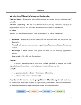
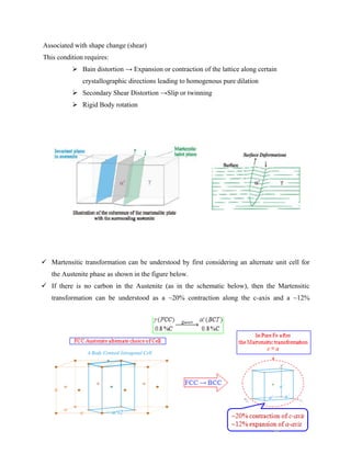
Solved Example: Consider a single crystal of BCC iron oriented such that a tensile stress is
applied along a [010] direction.
(a) Compute the resolved shear stress along a (110) plane and in a [111] direction when a tensile
stress of 52 MPa (7500 psi) is applied
(b) If slip occurs on a (110) plane and in a direction, and the critical resolved shear stress is
30 MPa (4350 psi), calculate the magnitude of the applied tensile stress necessary to initiate
yielding.
Solution:
Determine the value of the angle between the normal to the (110) slip plane (i.e., the [110]
direction) and the [010] direction using [u1v1w1] = [110], [u2v2w2] = [010] and the following
equation.










 
))((
cos 2
2
2
2
2
2
2
1
2
1
2
1
2121211
wvuwvu
wwvvuu

]111[


16










 
])0()1()0][()0()1()1[(
)0)(0()1)(1()0)(1(
cos 222222
1

Similarly determine the value of λ, the angle between and [010] directions as follows:
Then calculate the value of τ RSS using the following expression:
τ RSS = σ cosϕ cosλ
=(152 Mpa)(cos 45)(cos 54.7)
= 21.3 Mpa
= 13060 psi
Yield Strength σY:
Mpa
MPa
y 4.73
)7.54)(cos45(cos
30

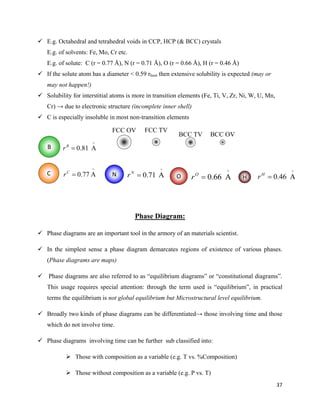
Plastic deformation by Twin:
 Twins are generally of two types: Mechanical Twins and Annealing twins
 Mechanical twins are generally seen in bcc or hcp metals and produced under conditions of
rapid rate of loading and decreased temperature.
 Annealing twins are produced as the result of annealing. These twins are generally seen in
fcc metals.
 Annealing twins are usually broader and with straighter sides than mechanical twins.
o
45)
2
1
(cos 1
 
]111[

o
7.54)
3
1
(cos
])0()1()0][()1()1()1[(
)0)(1()1)(1()0)(1(
cos 11
222222











 


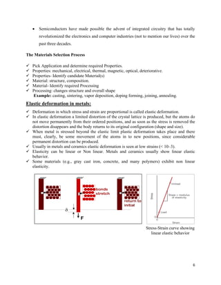
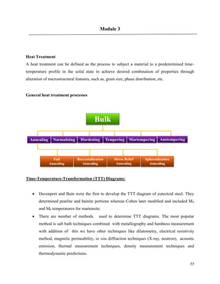
17
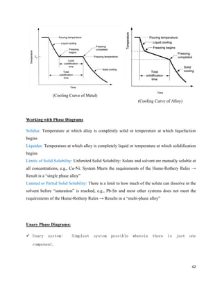
(a) Mechanical Twins (Neumann bands in iron), (b) Mechanical Twins in zinc produced by
polishing (c) Annealing Twins in gold-silver alloy
 Twinning generally occurs when the slip systems are restricted or when the slip systems are
restricted or when something increases the critical resolved shear stress so that the twinning
stress is lower than the stress for slip.
 So, twinning generally occurs at low temperatures or high strain rates in bcc or fcc metals or
in hcp metals.
 Twinning occurs on specific twinning planes and twinning directions.
Crystal
Structure
Typical
Examples
Twin Plane Twin Direction
BCC α-Fe, Ta (112) [111]
HCP
Zn, Cd,
Mg, Ti
FCC Ag, Au, Cu (111) [112]
(Twin planes and Twin directions)
)2110(

]0111[


18
Difference between in slip in Twin:
SLIP TWIN
 The crystallographic orientation above and
below the slip plane is the same both
before and after the deformation
 Slip occurs in distinct atomic spacing
multiples
 Slip Leaves a series of steps (lines)
 Normally slip results in relatively large
deformations
 Mostly seen in FCC and BCC structure, as
they have more slip systems
 Occurs on widely spread planes
 Orientation difference is seen across the
twin plane
 the atomic displacement for twinning is
less than the inter-atomic separation
 Twinning leaves small but well defined
regions of the crystal deformed
 Only small deformations result for
twinning
 Is most important for HCP structure,
because of its small number of slip
system
 Occurs on every plane of region involved
Plastic deformation of Polycrystalline Materials:
 Plastic deformation in polycrystalline materials is very complex than those in the single
crystals due to the presence of grain boundaries, different orientation of neighboring crystals,
presence of several phases etc.
 Due to random crystallographic orientations, the slip planes and slip direction varies from
one grain to another.
 As a result the resolved shear stress τRSS will vary from one crystal to another and the
dislocations will move along the slip systems with favorable orientation (i.e. the highest
resolved shear stress).

19
 When a polished polycrystalline specimen of copper is plastically deformed, two slip systems
operate for most of the grains (evidenced by two sets of parallel yet intersecting sets of lines).
 Slip lines are visible, and the variation in grain orientation is indicated by the difference in
alignment of the slip lines for several grains.
 During deformation, mechanical integrity and coherency are maintained along the grain
boundaries; i.e. the grain boundaries usually do not come apart or open up.
 As a consequence, each individual grain is constrained, to some degree in the shape it may
assume by its neighboring grains.
Alteration of the grain structure of a polycrystalline metal as a result of plastic deformation (a)
before deformation the grains are equiaxed. (b) after deformation elongated grains are produced
Slip lines

20
Strengthening Mechanisms
The ability of a metal to deform depends on the ability of the dislocations to move and the slip of
dislocations weakens the crystal. Hence we have two strategies to strengthen the crystal/material:
 completely remove dislocations  difficult, but dislocation free whiskers have been
produced (however, this is not a good strategy as dislocations can nucleate during
loading)
 Increase resistance to the motion of dislocations or put impediments to the motion of
dislocations  this can be done in many ways as listed below.
Solid Solution Strengthening:
 The introduction of solute atoms into solid solution in the solvent-atom lattice invariably
produces an alloy which is stronger than the pure metal.
 Two types of solid solutions:
 Substitutional solid solutions → Solute atoms occupy lattice points in the solvent
lattice (Hume Rothery’s rules are to be satisfied)
 Interstitial solid solutions → Solute atoms occupy interstitial positions in the solvent
lattice (Carbon, Nitrogen, Boron, Oxygen, Hydrogen are the common interstitial
solutes)
 Smaller solute atoms → Tensile stress field & Larger solute atoms → Compressive stress
field
 The stress fields around solute atoms interact with the stress fields around the dislocation.

21
 This interaction provides frictional resistance to dislocations motion and static locking of
dislocations
 The factors playing an important role on strengthening effect:
 Size of the solute
 Concentration of solute
 Elastic modulus of the solute (higher E → greater strengthening effect)
 Nature of solute atoms (Interstitial or substitutional)
Solute strengthening of Cu crystal
by solutes of different sizes
 More the size difference, more the
intensity of stress field around
solute atoms and more is the
hardening effect.
 Large the concentration of solute,
more obstacles to dislocations
motion and strength increases
(Increase in σY is proportional to
the square root of concentration of
the solute).
 Interstitial solute atoms can
elastically interact with both edge
and screw dislocations and results
in intense distortion compared to
that of substitutional atoms.
 Hence they give a higher
hardening effect (per unit
concentration) as compared to
substitutional atoms.

22
(Substitutional ) (Interstitial)
Hardening by precipitates and dispersoids:
 Small second-phase particles distributed in a ductile matrix can hinder the dislocation motion
and thus increase the strength of a material. Second-phase particles either can be introduced
by mixing and consolidation (dispersion strengthening) or precipitated in solid state
(precipitation hardening).
Precipitation hardening:
 Precipitation hardening or age hardening is produced by solution treating and quenching an
alloy. Term ‘Age hardening’ is used to describe the process because strength develops with
time.
 Requisite for precipitation hardening to take place is that second phase must be soluble at an
elevated temperature but precipitates upon quenching and aging at a lower temperature.
 Mostly seen in: Al-alloys, Cu-Be alloys, Mg-Al alloys, Cu-Sn alloys.
 Precipitates may be coherent, semi-coherent or incoherent. Coherent (& semi-coherent)
precipitates are associated with coherency stresses.
 If the precipitate is coherent with the matrix then Dislocations can glide through it. Glide of
the dislocation causes a displacement of the upper part of the precipitate w.r.t the lower part
by b → ~ cutting of the precipitate.

23
 Dislocations cannot glide through incoherent precipitates and widely separated inclusions.
Hence they bow around the widely separated inclusions. In this process they leave
dislocation loops around the inclusions, thus leading to an increase in dislocation density.
This is known as the Orowan bowing mechanism.

24
 The next dislocation arriving (similar to the first one), feels a repulsion from the dislocation
loop and hence the stress required to drive further dislocations increases. Additionally, the
effective separation distance (through which the dislocation has to bow) reduces from‘d’ to
‘d1’.
 Inclusions behave similar to incoherent precipitates in this regard (precipitates are part of the
system, whilst inclusions are external to the alloy system).
 A pinned dislocation (at a precipitate) has to either climb over it (which becomes favorable at
high temperatures) or has to bow around it.
Dispersion hardening:
 In dispersion hardening, the hard particles are mixed with matrix powder and consolidated
and processed by powder metallurgy techniques.
 Example: Thoria dispersed Nickel  Fine particles of Thoria are dispersed in the nickel
matrix and the inter particle distance is enough to hinder the dislocation movement thereby
increasing the strength up to 0.9 times Tm (Tm in 0
C).
 In dispersion hardening, dispersoids are incoherent with the matrix and dislocations cannot
glide through these dispersoids and gets pinned.
 A pinned dislocation (at a precipitate) has to either climb over it (which becomes favorable at
high temperatures) or has to bow around it (Orowan’s Mechanism of Dispersion Hardening)
 Dislocation loop exert a back stress on dislocation which needs to be overcome for additional
slip to take place and this causes hardening.

25
Strengthening by Grain Boundary:
 Grain boundary is the boundary between two grains in a polycrystalline aggregate and this is
the region of a disturbed lattice which is of few atomic diameters distance.
 There are two important ways in which grain boundary acts as a barrier to the dislocation
 Difficulty for a dislocation to pass through two different grain orientations (need to
change the direction)
 The atomic disorder within a grain boundary region contributes to a discontinuity of
slip planes from one grain to other.
 Hence dislocations are stopped by a grain boundary and pile up against it.
 A fine grained material is harder and stronger than one that is coarse grained since greater
amounts of grain boundaries in the fine grained materials impede dislocation motion.
 The general relationship between yield stress (tensile strength) and grain size was proposed by
Hall and Petch, which is known as Hall-Petch relation.

26
(Influence of grain size on yield strength of 70Cu-30Zn Brass)
Strain Hardening: Forest Dislocations:
 Increasing strength and hardness by plastic deformation is called strain hardening or work
hardening. Also referred as cold working as deformation takes place at room temperature.
 With plastic deformation dislocation density increases because under applied stress
dislocation sources, like Frank-Reed source, becomes active.
)1010(~)1010(~ 1412
ndislocatio
96
ndislocatio 
 
 
materialStrongermaterialAnnealed workCold
 Extent of strain hardening increases with degree of cold working (% area reduction).
 Since the metal is deformed in a certain direction, grains are elongated in the direction of
working.
 The consequence of strain hardening a material is improved strength and hardness but
material’s ductility will be reduced.
Mechanism:
 Cold working generates dislocations – dislocation density increases. Higher density of
dislocations impedes their motion due to interactions of dislocation strain fields.
 Hence the strength increases according to the relation: 2
1
 Ao  , where τ is the shear
stress to move a dislocation that increases with increase in dislocation density (ρ).
2
1

 dkyoYield 
Where,
σyield = Yield stress
σo = Friction stress or resistance
to dislocation motion
ky = Locking parameter or the
hardening contribution from the
grain boundary
d = Grain diameter

27
Cold Working & its effect on properties:
 Plastic deformation in the temperature range (0.3 – 0.5) Tm → Cold Work
 Point defects and dislocations have strain energy associated with them
 (1 -10) % of the energy expended in plastic deformation is stored in the form of strain energy
(in these defects) → The material becomes battery of energy….!
 The cold worked material is in a micro structurally metastable state.
 Depending on the severity of the cold work the dislocation density can increase 4-6 orders of
magnitude more. The material becomes stronger, but less ductile.
 In addition to mechanical properties, physical properties of a material also changes during
cold working. There is usually a small decrease in density, an appreciable decrease in
electrical conductivity, small increase in thermal coefficient of expansion and increased
chemical reactivity (decrease in corrosion resistance).
 Cold working is typically done on ductile metals (e.g. Al, Cu, Ni).
 Heating the material (typically below 0.5Tm) is and holding for sufficient time is a heat
treatment process called annealing.
 Depending on the temperature of annealing processes like Recovery at lower temperatures)
or Recrystallization (at higher temperatures) may take place. During these processes the
material tends to go from a micro structurally metastable state to a lower energy state
(towards a stable state).
 Further ‘annealing’ of the recrystallized material can lead to grain growth.
Recovery, Recrystallization and Grain Growth:
Annealing is an important industrial process to relieve the stresses from cold working. During
cold working grain shape changes, while material strain hardens because of increase in
dislocation density. Between 1-10% of the energy of plastic deformation is stored in material in
the form of strain energy associated with point defects and dislocations. On annealing i.e. on
heating the deformed material to higher temperatures and holding, material tends to lose the
extra strain energy and revert to the original condition before deformation by the processes of
recovery and recrystallization. Grain growth may follow these in some instances.

28
Recovery:
 Recovery takes place at low temperatures of annealing
 “Apparently no change in microstructure”
 Excess point defects created during Cold work are absorbed:
 At surface or grain boundaries
 By dislocation climb
 Random dislocations of opposite sign come together and annihilate each other.
 Dislocations of same sign arrange into low energy configurations ((POLYGONIZATION):
 Edge → Tilt boundaries
 Screw → Twist boundaries
 Overall reduction in dislocation density is small
 At the early stage of annealing of cold formed metals, external thermal energy permits the
dislocations to move and form the boundaries of a polygonized subgrain structure while the
dislocation density stays almost unchanged. This process also removes the residual stresses
formed due to cold working significant. The recovering of physical and mechanical
properties varies with the temperature and time.
Bent
crystal
Low angle grain
boundaries

29
Recrystallization:
 TRecrystallization  (0.3 – 0.5) Tm
 “Nucleation” and growth of new, strain free crystals
 Nucleation of new grains in the usual sense may not be present and grain boundary migrates
into a region of higher dislocation density
 G (recrystallization) = G (deformed material) – G (undeformed material)
 TRecrystallization is the temperature at which 50 % of the material recrystallizes in 1 hour
 There are many variables that influence recrystallization behavior, namely amount of prior
deformation, temperature, time, initial grain size, composition and amount of recovery prior
to the start of the recrystallization. This dependence leads to following empirical laws:
 Deformation ↑  recrystallization temperature (Trecrystallization) ↓
 Initial grain size ↓  recrystallization temperature ↓
 High cold work + low initial grain size  finer recrystallized grains
Direction of grain
boundary
migration
Region of higher
dislocation density
Region of lower
dislocation density

30
 ↑ cold work temperature  lower strain energy stored  ↑ recrystallization
temperature
 Rate of recrystallization = exponential function of temperature
 Trecrystallization = strong function of the purity of the material
Trecrystallization (very pure materials) ~ 0.3 Tm
Trecrystallization (impure) ~ (0.5 – 0.6) Tm
Trecrystallization (99.999% pure Al) ~ 75o
C
Trecrystallization (commercial purity) ~ 275o
C
 The impurity atoms segregate to the grain boundary and retard their motion →
Solute drag (can be used to retain strength of materials at high temperatures).
 Second phase particles also pin down the grain boundary during its migration .
Grain Growth:
 Large grains have lower free energy than small grains. This is associated with the reduction
of the amount of grain boundary.
 Therefore, under ideal conditions, the lower energy state for a metal would be as a single
crystal. This is driving force for grain growth.
 Opposing this force is the rigidity of the lattice. As the temperature increases, the rigidity of
the lattice decreases and the rate of grain growth is more rapid.
 At any given temperature there is a maximum grain size at which these two effects are in
equilibrium

31
Hot Work  Plastic deformation above TRecrystallization
Cold Work  Plastic deformation below TRecrystallization
When a metal is hot worked, the conditions of deformation are such that the sample is soft
and ductile. The effects of strain hardening are negated by dynamic and static processes
(which keep the sample ductile).
The lower limit of temperature for hot working is taken as 0.6 Tm

32
Module-1I
Constitution of Alloys:
Structure of metals and materials is the most important aspect as properties depend upon the
features of the materials.
Phase:
 Anything which is homogenous and physically distinct.
 It can also be defined as anything which is physically distinct, chemically homogeneous, and
mechanically separable.
 And it must be kept in mind that chemically homogeneity or uniformity does not mean on
atomic scale for alloy, such as composition of each unit cell. But it is on large scale.
 Any structure which is visible as physically distinct under microscope is called phase.
 For pure elements phase means the states of the metals:
 Solid state –solid phase
 Liquid state –liquid phase
 Gaseous state-gaseous phase.
 Certain metals show allotropic modification and change its crystal structure changing its
phase.
 Example of metals showing allotropic transformation: iron, tin, zirconium, titanium, tungsten
 Tin shows two allotropic modification
 Alpha tin (grey tin) → it exists below 13.2 degree centigrade
 Beta tin (white tin) → it exists above13.2 degree centigrade.
 Iron showing three allotropic transformation:
 Fcc (Atmospheric pressure) → gamma iron
 Bcc (Atmospheric pressure)
o delta iron, alpha iron, beta iron (beta iron is paramagnetic in nature where as
alpha iron ferromagnetic in nature)
o alpha iron is room temperature phase.

33
 Hcp (high pressure)
 In solid states three types of phases are possible to form: Pure Metal, Compound and Solid
Solution
Pure Metal:
 Sharp melting and freezing point under equilibrium condition.
 Cooling curve (Temp vs Time) of a pure metal shows a horizontal line at its melting or
freezing point.
Alloy:
 It a combination of two or more elements from which at least one is metal, the substance
formed will must showing properties of metals.
 Alloys are made by mixing the constituents in liquid state. Here one will be the host metal
and other is alloying elements.
 Example of alloys: plain carbon steels, alloy steels etc.
 Classification of alloy on basis of no of elements present:
 Binary alloy system-990 system possible
 Ternary alloy system-14000 system possible
 Alloys can also classified as
1. Homogeneous alloy (consist of single phase)
2. Heterogeneous alloy or mixture (consists of multiple or mixture of phases)
Alloy system
Homogeneous (Single phase) Heterogeneous alloy or mixture
1-solid solution
Solid solution are two types :
a-interstitial solid solution (ex-plain carbon
steel)
Any combination of solid phases; may be
combination of Pure metals , solid
solution, intermediate alloy

34
b-substitution solid solution
i-Order solid solution (form a regular
pattern of arrangements)
ii-Disorder solid solution (ex- nikel and
copper form monel alloy)
2-intermediate alloy phase (compound)
Compound or Intermediate Alloy Phase:
 Combination of two or more atoms in a definite proportion.
 Combination of positive and negative valence elements.
 After forming a compound the elements lose their individual identity and properties.
 Some compound behaves like pure metals having a definite melting point with narrow limits
of temperature. So cooling curve for a compound is similar to that of a pure metal. It is
referred to as a congruent melting phase.
 Chemical composition of intermediate alloy phase is intermediate between the two pure
metals and generally has crystal structure different from those of pure metals.
Intermetallic compounds
 If two elements have high difference in electronegetivity, they tend to from a system called
intermetallic compound.
 Intermetallic compounds like MgSe, PbSe, Mg2Si, Cu2S are cubic whereas NiAs, MnSe,
CuSn are hexagonal.
Electron or Hume Rothery phases
 These compounds have wide range of solubility and occur at certain values of valence
electrons to atom ratio such as 3:2
 (CuZn), 21:13 (Cu5Zn8), 7:4 (CuZn3).
Laves phase

35
 Laves phases have a general formula of AB2, for example MgCu2 (cubic), MgZn2
(hexagonal), MgNi2 (hexagonal)
Sigma phase
 Sigma phase has a very complex crystal structure and is very brittle. This phase can act as a
source of embrittlement in some alloys such as steels.
Metal carbides and nitrides
 Metals which have high chemical affinity for carbon and nitrogen form carbides and nitrides
such as VC, NbC, VN, NbN, TiC, TiN. They can act as source of hardening in many alloys.
Solid solution:
 It can be defined as a solution in solid state, which consists of two kinds of atoms combined
in one type of space lattice.
 Example: Austenite , ferrite, delta iron, martensite
 Solution may be solid, liquid or gaseous; Example – sugar or salt in water.
 Solution may consist of two parts one is major part called solvent and minor called solute.
 On the basis of dissolution capacity or amount of solute present in solution there possible
condition of solution are there :
1- Unsaturated
2- Saturated
3- Supersaturated.
 Solubility of solute is a function of temperature with pressure constant.
 Solid solution are of two types: Substitutional and Interstitial
Substitutional Solid Solution:
 In this type of solution, the atoms of the solute substitute for atoms of the solvent in the
lattice structure of the solvent.
 Several factors are now known, largely through the work of Hume-Rothery, that control the
range of solubility in alloy systems.

36
 Empirical rules for the formation of substitutional solid solution (Hume-Rothery’s Rule)
 Crystal structure factor: For complete solid solubility, the two elements should have the
same type of crystal structure i.e., both elements should have either F.C.C. or B.C.C. or
H.C.P. structure.
 Relative size factor: As the size (atomic radii) difference between two elements
increases, the solid solubility becomes more restricted. For extensive solid solubility the
difference in atomic radii of two elements should be less than about 15 percent. If the
relative size factor is more than 15 percent, solid solubility is limited. For example, both
silver and lead have F.C.C. structure and the relative size factor is about 20 percent.
Therefore the solubility of lead in solid silver is about 1.5 percent and the solubility of
silver in solid lead is about 0.1 percent. Copper and nickel are completely soluble in each
other in all proportions. They have the same type of crystal structure (F.C.C.) and differ
in atomic radii by about 2 percent.
 Chemical affinity factor: Solid solubility is favoured when the two metals have lesser
chemical affinity. If the chemical affinity of the two metals is greater then greater is the
tendency towards compound formation. Generally, if the two metals are separated in the
periodic table widely then they possess greater chemical affinity and are very likely to
form some type of compound instead of solid solution.
 Relative valence factor: It is found that a metal of lower valence tends to dissolve more of
a metal of higher valence than vice versa. For example in aluminium-nickel alloy system,
nickel (lower valance) dissolves 5 percent aluminium but aluminium (higher valence)
dissolves only 0.04 percent nickel.
 Solid solutions which have a negative enthalpy of mixing (Hmix < 0) prefer unlike nearest
neighbours → show tendency for ordering and forms order solid solution.
 Solid solutions which have a positive enthalpy of mixing (Hmix > 0) forms clusters of same
types of atoms → Forms disorder solid solution.
 Solid solutions with zero enthalpy of mixing (Hmix = 0) forms ideal solution.
Interstitial Solid Solution:
 The second species added goes into the voids of the parent lattice

37
 E.g. Octahedral and tetrahedral voids in CCP, HCP (& BCC) crystals
E.g. of solvents: Fe, Mo, Cr etc.
E.g. of solute: C (r = 0.77 Å), N (r = 0.71 Å), O (r = 0.66 Å), H (r = 0.46 Å)
 If the solute atom has a diameter < 0.59 rhost then extensive solubility is expected (may or
may not happen!)
 Solubility for interstitial atoms is more in transition elements (Fe, Ti, V, Zr, Ni, W, U, Mn,
Cr) → due to electronic structure (incomplete inner shell)
 C is especially insoluble in most non-transition elements
Phase Diagram:
 Phase diagrams are an important tool in the armory of an materials scientist.
 In the simplest sense a phase diagram demarcates regions of existence of various phases.
(Phase diagrams are maps)
 Phase diagrams are also referred to as “equilibrium diagrams” or “constitutional diagrams”.
This usage requires special attention: through the term used is “equilibrium”, in practical
terms the equilibrium is not global equilibrium but Microstructural level equilibrium.
 Broadly two kinds of phase diagrams can be differentiated→ those involving time and those
which do not involve time.
 Phase diagrams involving time can be further sub classified into:
 Those with composition as a variable (e.g. T vs. %Composition)
 Those without composition as a variable (e.g. P vs. T)

38
 Time-Temperature-Transformation (TTT) diagrams and Continuous-Cooling-Transformation
(CCT) diagrams involve time. These diagrams will be considered in the chapter on Heat
treatment.
Some Important definitions:
Phase:
 A physically homogeneous and distinct portion of a material system (e.g. gas, crystal,
amorphous etc.)
 Gases: Gaseous state always a single phase → mixed at atomic or molecule level.
 Liquids: Liquid solution is a single phase → e.g. Nacl in H2O and Liquid mixtures consists
of two or more phases → e.g. Oil in water (no mixing at the atomic level)
 Solids: In general due to several compositions and crystals structures many phases are
possible.
 For the same composition different crystal structures represent different phases. E.g. Fe
(BCC) and Fe (FCC) are different phases.
Components of a system:
 Independent chemical species which comprise the system. These could be Elements, Ions,
and Compounds.
 Example: Au-Cu system : Components →Au, Cu (elements)
Ice-water system: Component→H2O (compound)
Al2O3-Cr2O3 system: Components→ Al2O3, Cr2O3
What kinds of phases exist?
 Based on state → Gas, Liquid, Solid
 Based on atomic order → Amorphous, Quasi-crystalline, Crystalline
 Based on band structure → Insulating, Semi-conducting, Semi-metallic, Metallic
 Based on Property → Para-electric, Ferromagnetic, Superconducting
 Based on stability → Stable, Metastable, Unstable
 Also sometimes- Based on size/geometry of an entity → Nanocrystalline, mesoporous,
layered.

39
Phase transformation:
 Phase transformation is the change of one phase into another. For example
 Water → Ice and α-Fe (BCC) → γ-Fe (FCC)
Grain:
 The single crystalline part of polycrystalline metal separated by similar entities by a grain
boundary.
Microstructure:
 (Phases + defects + residual stress) & their distributions
 Structures requiring magnifications in the region of 100 to 1000 times. (or) The distribution
of phases and defects in a material.
Variables/Axis of phase diagrams:
 The axes can be:
 Thermodynamic (T, P, V)
 Kinetic (t) or Composition variables (C, %X)
 In single component systems (unary systems) the usual variables are T & P
 In phase diagrams used in materials science the usual variable are T & %X
 In the study of phase transformation kinetics TTT diagrams or CCT diagrams are also used
where the axis are T & t
Degree of Freedom:
The degree of freedom, F, are those externally controllable conditions of temperature, pressure,
and composition, which are independently variable and which must be specified in order to
completely define the equilibrium state of the system.

40
Phase Rule:
 The phase rule connects the Degrees of Freedom, the number of components in a system and
the number of phases present in a system via a simple equation: F = C – P + 2, where C – No.
of components, P – No. of phases and F – No. of degrees of freedom
 The degrees of freedom cannot be less than zero so that we have an upper limit to the number
of phases that can exist in equilibrium for a given system.
Variation of the number of degrees of freedom with number of components and number of
phases:
Experimental Methods for Determination of Phase Diagram:
Metallography methods:
 It is microscopic observation of metallic samples (alloys)
 Metallo- metals alloys & Graphy-images
 In this methods heating the sample (alloy)to different temperature when equilibrium between
phases is established then it is cooled quickly to retained the high temperature structure.
 Limitation :
1-rapid cooling samples from high temperature do not allow retaining their high
temperature structure.
2-very difficult to interpret the observed microstructure excellent skill is required.
X ray diffraction:

41
 It studies the lattice dimension or measure the lattice dimension, so it indicates the
appearance of a new phase either by the change in the lattice dimension or by appearance of
the new crystal structure.
 Since for different phase the value of a is different to determine the value of a we have to
find out the value of d.
 d= a/(h2
+ k2
+ l2
)1/2
 This method is simple, precise very useful tool to determine the changes in the solid
solubility with temperature.
Thermal analysis:
 Here temperature vs time at constant composition plot (Cooling Curve) is drawn. It shows a
change in the slope at the point where there is a phase transformation occurs due to evolution
or absorption of heat.
 By this method we can determine initial and final temperature of solidification so it is a best
method for this but not a best methods to determine the phase transformation as very less
amount of heat change occurs during the solid state phase transformation.
Cooling curve:
 It’s a plot between temperature and time.
 Cooling curves gives us idea about the solidification start and end temperature.
 Since a metal is having a sharp melting and freezing temperature we will get a horizontal line
for the cooling curve. And since alloy has a range of melting temperature we will get a
curved cooling curved. So for the pure metals beginning and end of the solidification occurs
at a constant temperature.

42
(Cooling Curve of Metal)
(Cooling Curve of Alloy)
Working with Phase Diagrams
Solidus: Temperature at which alloy is completely solid or temperature at which liquefaction
begins
Liquidus: Temperature at which alloy is completely liquid or temperature at which solidification
begins
Limits of Solid Solubility: Unlimited Solid Solubility: Solute and solvent are mutually soluble at
all concentrations, e.g., Cu-Ni. System Meets the requirements of the Hume-Rothery Rules →
Result is a “single phase alloy”
Limited or Partial Solid Solubility: There is a limit to how much of the solute can dissolve in the
solvent before “saturation” is reached, e.g., Pb-Sn and most other systems does not meet the
requirements of the Hume-Rothery Rules → Results in a “multi-phase alloy”
Unary Phase Diagrams:
 Unary system: Simplest system possible wherein there is just one
component.

43
 Though there are many possibilities even in unary phase diagram (in terms
of the axis and phases), we shall only consider a T-P unary phase diagram.
 Let us consider the water (H2O) unary phase diagram
 The Gibbs phase rule here is: F=C-P+2 (2 is for T&P) (no composition
variables here)
 Along the 2 phase co-existence (at B & C) lines the degree of freedom (F)
is 1 → i.e. we can chose either T or P and the other will be automatically
fixed.
 The 3 phase co-existence points (at A) are invariant points with F=0.
(Invariant point implies they are fixed for a given system).
 The single phase region at point D, T and P can both be varied while still
being in the single phase region with F = 2.
(Phase diagram for water) (Phase diagram for pure iron)
Binary Phase Diagrams:
 Binary implies that there are two components.
 Pressure changes often have little effect on the equilibrium of solid phases (unless of course
we apply ‘huge’ pressures).

44
 Hence, binary phase diagrams are usually drawn at 1 atmosphere pressure.
 The Gibbs phase rule is reduced to: Variables are reduced to: F = C – P + 1 (1 is for T).
 T & Composition (these are the usual variables in materials phase diagrams)
 Binary phase diagrams can be classified based on:
 Complete solubility in both liquid & solid states
 Complete solubility in both liquid state, but limited solubility in the solid state
 Limited solubility in both liquid & solid states
Isomorphous Phase Diagram:
 Isomorphous phase diagrams form when there is complete solid and liquid solubility.
 Complete solid solubility implies that the crystal structure of the two components has to be
same and Hume-Rothery rules are to be followed.
 Examples of systems forming isomorphous systems: Cu-Ni, Ag-Au, Ge-Si, Al2O3-Cr2O3
 Both the liquid and solid contain the components A and B.

45
 In binary phase diagrams between two single phase regions there will be a two phase region
→ in the isomorphous diagram between the liquid and solid state there is the (Liquid + Solid)
state.
 The Liquid + Solid state is NOT a semi-solid state → it is a solid of fixed composition and
structure, in equilibrium with a liquid of fixed composition.
 In some systems (e.g. Au-Ni system) there might be phase separation in the solid state (i.e.
the complete solid solubility criterion may not be followed) → these will be considered as a
variation of the isomorphous system (with complete solubility in the solid and the liquid
state.
 In the Cu-Ni isomorphous diagram shown below; the single phase regions have degree of
freedom=2 i.e. T and Composition can both be varied while still being in the single phase
region. In the two phase region, if we fix T (and hence exhaust our DOF), the composition of
liquid and solid in equilibrium are automatically fixed (i.e. we have no choice over them).
Alternatively we can use our DOF to choose Cl then T and Cs are automatically fixed.
(Cooling Curve: Isomorphous System) (Cu-Ni isomorphous phase diagram)
Chemical Composition of Phases:

46
 To determine the actual chemical composition of the phases of an alloy, in equilibrium at any
specified temperature in a two phase region, draw a horizontal temperature line, called a tie
line, to the boundaries of the field.
 These points of intersection are dropped to the base line, and the composition is read directly.
Relative Amounts of Each Phase:
 To determine the relative amounts of the two phases in equilibrium at any specified
temperature in a two phase region, draw a vertical line representing the alloy and a horizontal
temperature line to the boundaries of the field.
 The relative lengths of the lever arms multiplied by the amounts of the phases present must
balance.
Tie line and Lever rule
 We draw a horizontal line (called the Tie Line)at the temperature of interest (say T0). Let Tie
line is XY.
 Solid (crystal) of composition C 1 coexists with
liquid of composition C 2
 Note that tie lines can be drawn only in the two
phase coexistence regions (fields). Though they
may be extended to mark the temperature.
 To find the fractions of solid and liquid we use the
lever rule.
 The portion of the horizontal line in the two phase region is akin to ‘lever’ with the fulcrum
at the nominal composition (C0)
 The opposite arms of the lever are proportional to
the fraction of the solid and liquid phase present

47
Variations of Isomorphous System:
 An alloy typically melts over a range of temperatures. However, there are special
compositions which can melt at a single temperature like a pure metal. There is no difference
in the liquid and solid composition. It begins and ends solidification at a constant temperature
with no change in composition, and its cooling curve will show a horizontal line.
 Such alloys are known as congruent-melting alloys, sometimes known as a pseudo-eutectic
alloy. Ex: Cu-Au, Ni-Pd.

48
 Elevation in the MP means that the solid state is ‘more stable’ (crudely speaking the ordered
state is more stable) → ordering reaction is seen at low T.
 Depression in MP ‘means’ the liquid state (disordered) is more stable → phase separation is
seen at low T. (phase separation can be thought of as the opposite of ordering. Ordering
(compound formation) occurs for –ve values for ΔH mix).
Equilibrium Cooling:

49
(Slow cooling, under equilibrium conditions, of a particular alloy 70A-30B)
 This alloy at temperature T0 is a homogeneous single-phase liquid solution (a) and remains
so until temperature T1is reached. Since T1is on the liquidus line, freezing or solidification
now begins.
 The first nuclei of solid solution to form α1 will be very rich in the higher melting point metal
A and will be composed of 95A-5B (by tie line rule). Since the solid solution in forming
takes material very rich in A from the liquid, the liquid must get richer in B. Just after the
start of solidification, the composition of the liquid is approximated as 69A-31B (b).
 When the lower temperature T2 is reached, the liquid composition is at L2. The only solid
solution in equilibrium with L2 and therefore the only solid solution forming at T2 is α2.
Applying tie line rule, α2 is composed of 10B. Hence, as the temperature is decreased, not
only does the liquid composition become richer in B but also the solid solution.
 At T2, crystals of α2 are formed surrounding the α1 composition cores and also separate
dendrites of αz (see figure in below).
 In order for equilibrium to be established at T2, the entire solid phase must be a composition
α2. This requires diffusion of B atoms to the A-rich core not only from the solid just formed
but also from the liquid. This is possible in crystal growth (c).
 The composition of the solid solution follows the solidus line while the composition of liquid
follows the liquidus line, and both phases are becoming richer in B.
 At T3 (d), the solid solution will make up approximately three-fourths of all the material
present.

50
 Finally, the solidus line is reached at T4, and the last liquid L4, very rich in B, solidifies
primarily at the grain boundaries (e).
 However, diffusion will take place and all the solid solution will be of uniform composition
α(70A-30B), which is the overall composition of the alloy (f).
 There are only grains and grain boundaries. There is no evidence of any difference in
chemical composition inside the grains, indicating that diffusion has made the grain
homogeneous.
Non Equilibrium Cooling:
 In actual practice it is extremely difficult to cool under equilibrium conditions. Since
diffusion in the solid state takes
place at a very slow rate, it is
expected that with ordinary cooling
rates there will be some difference
in the conditions as indicated by
the equilibrium diagram.

51
 Consider again 70A-30B alloy, solidification starts at T1 forming a solid solution of
composition α1 .
 At T2 the liquid is L2 and the solid solution now forming is of composition α2 . Since
diffusion is too slow to keep pace with crystal growth, not enough time will be allowed to
achieve uniformity in the solid, and the average composition will be between α1 and α2, say
α’2.
 As the temperature drops, the average composition of the solid solution will depart still
further from equilibrium conditions. It seems that the composition of the solid solution is
following a “nonequilibrium” solidus line α1 to α’5, shown dotted lines in the figure.
 The liquid, on the other hand, has essentially the composition given by the liquidus line,
since diffusion is relatively rapid in liquid. At T3 the average solid solution will be of
composition α’3 instead of α3.
 Under equilibrium cooling, solidification should be complete at T4 ; however, since the
average composition of the solid solution α’4 has not reached the composition of the alloy,
some liquid must still remain. Applying lever rule at T4 gives α’4 = 75% and L4 = 25%.
 Therefore, solidification will continue until T5 is reached. At this temperature the
composition of the solid solution α’5 coincides with the alloy composition, and solidification
is complete. The last liquid to solidify, L5, is richer in B than the last liquid to solidify under
equilibrium conditions.
 The more rapidly the alloy is cooled the greater will be the composition range in the
solidified alloy. Since the rate of chemical attack varies with composition, proper etching
will reveal the dendritic structure microscopically (see below figure). The final solid consists
of a “cored” structure with a higher-melting central portion surrounded by the lower-
melting, last-to-solidify shell. The above condition is referred to as coring or dendritic
segregation.
 To summarize, nonequilibrium cooling results in an increased temperature range over which
liquid and solid are present; Since diffusion has not kept pace with crystal growth, there will

52
be a difference in chemical composition from the center to the outside of the grains. The
faster the rate of cooling, the greater will be the above effects.
Eutectic Phase Diagram:
 Very few systems exhibit an isomorphous phase diagram (usually the solid solubility of one
component in another is limited).
 Often the solid solubility is severely limited – through the solid solubility is never zero (due
to entropic reasons).
 In a Simple eutectic system (binary), there is one composition at which the liquid freezes at a
single temperature. This is in some sense similar to a pure solid which freezes at a single
temperature (unlike a pure substance the freezing produces a two solid phases both of which
contain both the components).
 The term Eutectic means easy melting → The alloy of eutectic composition freezes at a
lower temperature than the melting point s of the constituent components.

53
 This has important implifications → e.g. the Pb-Sn eutectic alloy melts at 183 ºC, which is
lower than the melting points of both Pb (327ºC) and Sn (232ºC) → Can be used for
soldering purposes (as we want to input least amount of heat to solder two materials).
Microstructural Characteristics of Eutectic System:
 To
reiterate an
important
point:
Phase
diagram

54
do not contain microstructural information (i.e. they cannot tell you what the microstructures
produced by cooling is. Often microstructural information is overlaid on phase diagram for
convenience. Hence, strictly cooling is not in the domain of phase diagram – but we can
overlay such information keeping in view the assumptions involved.
Application of Lever rule in Eutectic System:
SOLVED EXAMPLE: For a 40 wt% Sn-60 wt% Pb alloy at 150°C, find the phases
present: α and β, Composition of phases.
Peritectic Phase Diagram:

55
 Like the eutectic system, the Peritectic reaction is found in systems with complete liquid
solubility but limited solid solubility.
 In the Peritectic reaction the liquid (L) reacts with one solid (α) to produce another solid (β).
L+α → β
 Since the solid β forms at the interface between the L and α, further reaction is dependent on
solid state diffusion. Needless to say this becomes the rate limiting step and hence it is
difficult to ‘equilibrate’ peritectic reactions (as compared to say eutectic reactions).
 In some Peritectic reactions (e.g. the Pt-Ag system – previous page). The (pure) β phase is
not stable below the Peritectic temperature (TP = 1186 ºC for Pt- Ag system) and splits into a
mixture of (α+β) just below TP.
Monotectic Phase Diagram:
 In all the types discussed previously, it was assumed that there was complete solubility in the
liquid state. It is quite possible, however, that over a certain composition range two liquid
solutions are formed that are not soluble in each other.

56
 Another term for solubility is miscibility. Substances that are not soluble in each other, such
as oil and water, are said to be immiscible. Substances that are partly soluble in each other
are said to show a miscibility gap, and this is related to Monotectic Systems.
 When one liquid forms another liquid, plus a solid, on cooling, it is known as a Monotectic
Reaction.
 It should be apparent that the Monotectic reaction resembles the eutectic reaction, the only
difference being that one of the products is a liquid phase instead of a solid phase.
 An example of an alloy system showing a Monotectic reaction is that between copper and
lead given in next page. Notice that in this case the L1 + L2 is closed.
 Also, although the terminal solids are indicated as α and β, the solubility is actually so small
that they are practically the pure metals, copper and lead.
Eutectoid Reaction:
 This is a common reaction in the solid state. It is very similar to the eutectic reaction but does
not involve the liquid . In this case, a solid phase transforms on cooling into two new solid
phases. The general equation may be written as..!

57
 The resultant Eutectoid mixture is extremely fine, just like the eutectic mixture. Under the
microscope both mixtures generally appear the same, and it is not possible to determine
microscopically whether the mixture resulted from a eutectic reaction or eutectoid reaction.
 An equilibrium diagram of Cu-Zn, illustrating the eutectoid reaction is shown in figure.
 In copper (Cu) – Zinc (Zn) system contains two terminal solid solutions i.e. these are extreme
ends of phase diagram α and η, with four intermediate phases called β, γ, δ and ε. The β’
phase is termed an ordered solid solution, one in which the copper and zinc atoms are
situated in a specific and ordered arrangement within each unit cell.
 In the diagram, some phase boundary lines near the bottom are dashed to indicate that there
positions have not been exactly determined. The reason for this is that at low temperatures,
diffusion rates are very slow and inordinately long times are required for the attainment of
equilibrium.
 Again only single- and two- phase regions are found on the diagram, and the same and we
can utilize the lever rule for computing phase compositions and relative amounts.

58
 The commercial material brasses are copper-rich copper-zinc alloys: for example, cartridge
brass has a composition of 70 wt% Cu-30 wt% Zn and a microstructure consisting of a single
α phase.
The Peritectoid Reaction:
 This is a fairly common reaction in the solid state and appears in many alloy systems. The
peritectoid reaction may be written as
 The new solid phase is usually an intermediate alloy, but it may also be a solid solution .The
peritectoid reaction has the same relationship to the peritectic reaction as the eutectoid has to
the eutectic. Essentially, it is the replacement of a liquid by a solid.
 The peritectoid reaction occurs entirely in the solid state and usually at lower temperatures
than the peritectic reaction, the diffusion rate will be slower and there is less likelihood that
equilibrium structures will be reached.
 Consider Silver (Ag) – Aluminium (Al) phase diagram (in next page) containing a peritectoid
reaction.

59
 If a 7% Al alloy is rapidly cooled from the two phase area just above the peritectoid
temperature the two phases will be retained, and the microstructure will show a matrix of γ
with just a few particles of α. When we cool at below the peritectoid temperature by holding
we get single phase μ.
Monotectoid Reaction : Al-Zn Phase Diagram

60
Syntectic Reaction : Ga – I Phase Diagram

61
Summary of Invariant reactions
Allotropic Transformations
 As we discussed earlier that several metals may exist in more than one type of crystal
structure depending upon temperature , Iron, Tin, Manganese and Cobalt are examples of
metals which exhibit this property , known as Allotropy.
 On an equilibrium diagram, this allotropic change is indicated by a point or points on the
vertical line which represents the pure metal. This is illustrated in below figure. In this
diagram, the gamma solid solution field is ‘looped’. The pure metal Fe and alloys rich in Fe
undergo two transformations.

62
Order-disorder Transformations
 Ordinarily in the formation of substitutional type of solid solution the solute atoms do not
occupy any specific position but are distributed at random in the lattice structure of the
solvent. The alloy is said to be in a ‘disordered’ condition.
 Some of these random solid solutions, if cooled slowly, undergo a rearrangement of the
atoms where the solute atoms move into definite positions in the lattice. This structure is
known as an ordered solid solution or superlattice.
 Ordering is most common in metals that are completely soluble in the solid state, and usually
the maximum amount of ordering occurs at a simple atomic ratio of the two elements.
 For this reason, the ordered phase is sometimes given a chemical formula, such as AuCu and
AuCu3 in the gold-copper alloy system. On the equilibrium diagram, the ordered solutions
are frequently designated as α‫׳‬ , β‫׳‬ , etc. or α‫׳‬ , α‫״‬ , etc., and the area in which they are found
is usually bounded by a dot-dash line.

63
 When the ordered phase has the same lattice structure as the disordered phase, the effect of
ordering on mechanical properties is negligible. Hardening associated with the ordering
process is most pronounced in those systems where the shape of the unitcell is changed by
ordering.
 Regardless of the structure formed as a result of ordering, an important property change
produced, even in the absence of hardening, is a significant reduction in electrical resistance.
Notice the sharp decrease in electrical resistivity at the compositions which correspond to the
ordered phases
AuCu and
AuCu3.
Allotropic
Transformations in Iron:
 Iron is an allotropic metal, which means that it can exist in more than one type of lattice
structure depending upon temperature. A cooling curve for pure iron is shown below:

64
o
Iron – Cementite Phase Diagram
 The Fe-C (or more precisely the Fe-Fe3C) diagram is an important one. Cementite is a
metastable phase and ‘strictly speaking’ should not be included in a phase diagram. But the
decomposition rate of cementite is small and hence can be thought of as ‘stable enough’ to be
included in a phase diagram. Hence, we typically consider the Fe-Fe3C part of the Fe-C
phase diagram.
 A portion of the Fe-C diagram – the part from pure Fe to 6.67 wt.% carbon (corresponding to
cementite, Fe3C) – is technologically very relevant.
 Cementite is not a equilibrium phase and would tend to decompose into Fe and graphite. This
reaction is sluggish and for practical purpose (at the microstructural level) cementite can be
considered to be part of the phase diagram. Cementite forms as it nucleates readily as
compared to graphite.
 Compositions upto 2.1%C are called steels and beyond 2.1% are called cast irons. In reality
the calssification should be based on ‘castability’ and not just on carbon content.
 Heat treatments can be done to alter the properties of the steel by modifying the
microstructure → we will learn about this in coming chapters.

66
(Iron – Cementite Phase Diagram)
Carbon Solubility in Iron:
Solubility of carbon in Fe = f (structure, temperature)
Where is carbon located in iron lattice?
Characteristics of phases appeared in Fe-Fe3C phase diagram:
Ferrite (α)
 It is an interstitial solid solution of a small amount of carbon
dissolved in α iron.
 The maximum solubility is 0.025%C at 723ºC and it dissolves only
0.008%C at room temperature. It is the softest structure that appears
on the diagram
 The crystal structure of ferrite (α) is B.C.C
 Tensile strength – 40,000 psi or 275 Mpa
 Elongation – 40% in 2 in.
 Hardness - < 0 HRC or < 90 HRB

67
Cementite (Fe3C)
 Cementite or iron carbide, chemical formula Fe3C, contains 6.67%C by weight and it is a
metastable phase.
 It is typically hard and brittle interstitial compound of low tensile strength (approx. 5000 psi)
but high compressive strength.
 It is the hardest structure that appears on the diagram.
 Its crystal structure is orthorhombic
Pearlite ( + Fe3C)
 Pearlite is the eutectoid mixture containing 0.80 %C and is formed at 723ºC on very slow
cooling.
 It is very fine plate-like or lamellar mixture
of ferrite and cementite. The fine fingerprint
mixture called pearlite is shown in below
figure.
 Elongation – 20 percent in 2 in.
 Hardness – HRC 20, HRB 95-100, or BHN 250-300
Austenite (γ)

68
 It is an interstitial solid solution of a small amount of carbon dissolved in γ iron. The
maximum solubility is 2.1%C at 1147ºC.
 The crystal structure of Austenite (γ) is F.C.C
 Elongation – 10% in 2 in.
 Hardness - 40 HRC and Toughness is high.
Ledeburite (γ+ Fe3C)
 Ledeburite is the eutectic mixture of austenite and cementite.
 It contains 4.3%C and is formed at 1147ºC
 Structure of ledeburite contains small islands of austenite are
dispersed in the carbide phase.
 Not stable at room temperature
Ferrite (δ)
 Interstitial solid solution of carbon in iron of body
centered cubic crystal structure. (δ iron ) of higher
lattice parameter (2.89Å) having solubility limit of
0.09 wt% at 1495°C with respect to austenite.
The stability of the phase ranges between 1394-
1539°C.
 This is not stable at room temperature in plain
carbon steel. However it can be present at room temperature in alloy steel especially duplex
stainless steel.
Microstructures involved in eutectoid mixture/Eutectoid reaction:

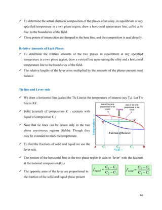
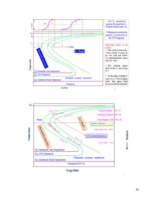
69
 Phase changes that occur upon passing from the γ
region into the α+ Fe3C phase field.
 Consider, for example, an alloy of eutectoid
composition (0.8%C) as it is cooled from a temperature
within the γ phase region, say 800ºC – that is, beginning
at point ‘a’ in figure and moving down vertical xx’.
Initially the alloy is composed entirely of the austenite
phase having composition 0.8 wt.% C and then
transformed to α+ Fe3C [pearlite]
 The microstructure for this eutectoid steel that is slowly
cooled through eutectoid temperature consists of
alternating layers or lamellae of the two phases α and Fe3C.
 The pearlite exists as grains, often termed “colonies”; within each colony the layers are
oriented in essentially the same direction, which varies from one colony to other.
 The thick light layers are the ferrite phase, and the cementite phase appears as thin lamellae
most of which appear dark.

70
Microstructures involved in Hypo eutectoid region:
 Hypo eutectoid region – 0.008 to 0.8 %C
 Consider vertical line yy’ in figure, at about
875ºC, point c, the microstructure will consist
entirely of grains of the γ phase.
 In cooling to point d, about 775ºC, which is
within the α+γ phase region, both these phases
will coexist as in the schematic microstructure
Most of the small α particles will form along the
original γ grain boundaries.
 Cooling from point d to e, just above the
eutectoid but still in the α+γ region, will produce
an increased fraction of α phase and a
microstructure similar to that also shown: the α
particles will have grown larger.
 Just below the eutectoid temperature, at point f, all the γ phase that was present at
temperature e will transform pearlite. Virtually there is no change in α phase that existed at
point e in crossing the eutectoid temperature – it will normally be present as a continuous
matrix phase surrounding the isolated pearlite colonies.
 Thus the ferrite phase will be present both in the pearlite and also as the phase that formed
while cooling through the α+γ phase region. The ferrite that is present in the pearlite is called
eutectoid ferrite, whereas the other, is termed proeutectoid (meaning pre- or before eutectoid)
ferrite.

71
Microstructures involved in Hypo eutectoid region:
 Hyper eutectoid region – 0.8 to 2.1 %C
 Consider an alloy of composition C1 in figure
that, upon cooling, moves down the line zz’. At
point g only the γ phase will be present and the
microstructure having only gamma grains.
 Upon cooling into the γ+ Fe3C phase field – say
to point h – the cementite phase will began to
form along the initial γ grain boundaries,
similar to the α phase in point d. this cementite is
called proeutectoid cementite that which forms
before the eutectoid reaction.
 As the temperature is lowered through the
eutectoid to point I, all remaining austenite of
eutectoid composition is converted into pearlite; thus the resulting microstructure consists of
pearlite and proeutectoid cementite as micro constituents.

72
Application of Lever rule in Fe-Fe3C phase diagr

73
Critical temperature lines:
 In general, A0 – Subcritical temperature, A1 - lower critical temperature, A3 - upper critical
temperature, A4 – Eutectic temperature, A5 – Peritectic temperature and Acm - γ/γ+cementite
phase field boundary.
 While heating we denoted as Ac1, Ac2, Ac3 etc., ‘c’ stands for chauffage (French word),
which means heating and while cooling we denoted as Ar1, Ar2, Ar3 etc., ‘r’ stands for
refroidissement, (French word) which means cooling.
Martensitic Transformations:
Under slow cooling rates, the carbon atoms are able to diffuse out of the austenite structure and it
leads to gamma to alpha transformation. This process involves nucleation and growth and it is
time dependent.
With a still further increase in cooling rate, insufficient time is allowed for the carbon to diffuse
out of solution, and although some movement of the iron atoms takes place, the structure cannot
become B.C.C. while the carbon is trapped in solution.
The resultant structure is called Martensite, is a supersaturated solid solution of carbon trapped
in a body-centered tetragonal structure and it is a metastable phase.
The highly distorted lattice structure is the prime reason for the high hardness of martensite.
After drastic cooling, martensite appears microscopically as a white needlelike or acicular
structure or lenticular, sometimes described as pile of straw.
Shape of the Martensite formed →Lenticular (or thin parallel plates)

74
Associated with shape change (shear)
This condition requires:
 Bain distortion → Expansion or contraction of the lattice along certain
crystallographic directions leading to homogenous pure dilation
 Secondary Shear Distortion →Slip or twinning
 Rigid Body rotation
 Martensitic transformation can be understood by first considering an alternate unit cell for
the Austenite phase as shown in the figure below.
 If there is no carbon in the Austenite (as in the schematic below), then the Martensitic
transformation can be understood as a ~20% contraction along the c-axis and a ~12%

75
expansion of the a-axis → accompanied by no volume change and the resultant structure has
a BCC lattice (the usual BCC-Fe) → c/a ratio of 1.0.
 In the presence of Carbon in the octahedral voids of CCP (FCC) -Fe (as in the schematic
below) → the contraction along the c-axis is impeded by the carbon atoms. (Note that only a
fraction of the octahedral voids are filled with carbon as the percentage of C in Fe is small).
 However the a1 and a2 axis can expand freely. This leads to a product with c/a ratio (c’/a’) >1
 In this case there is an overall increase in volume of ~4.3% (depends on the carbon content)
→ the Bain distortion.
 The Martensitic transformation occurs without composition change
 The transformation occurs by shear without need for diffusion and is called diffusion less
transformation
 The atomic movements (shearing) required are only a fraction of the inter atomic spacing
 The shear changes the shape of the transforming region
→ results in considerable amount of shear energy
→ plate-like shape of Martensite
 The amount of martensite formed is a function of the temperature to which the sample is
quenched and not of time
 Hardness of martensite is a function of the carbon content → but high hardness steel is very
brittle as martensite is brittle
 Steel is reheated to increase its ductility → this process is called TEMPERING

76
 The martensite transformation, for many years, was believed to be unique for steel. However,
in recent years, this martensite type of transformation has been found in a number of other
alloy systems, such as iron-nickel, copper-zinc, and copper-aluminum.
 The basic purpose of hardening is to produce a fully martensitic structure, and the minimum
cooling rate (per second) that will avoid the formation of any of the softer products of
transformation is known as the critical cooling rate.
 The critical cooling rate, determined by chemical composition and austenitic grain size, is an
important property of steel since it indicates how fast steel must be cooled in order to form
only martensite.

77
Module 3
Heat Treatment
A heat treatment can be defined as the process to subject a material to a predetermined time-
temperature profile in the solid state to achieve desired combination of properties through
alteration of microstructural features, such as, grain size, phase distribution, etc.
General heat treatment processes
Time-Temperature-Transformation (TTT) Diagrams:
 Davenport and Bain were the first to develop the TTT diagram of eutectoid steel. They
determined pearlite and bainite portions whereas Cohen later modified and included MS
and MF temperatures for martensite.
 There are number of methods used to determine TTT diagrams. The most popular
method is salt bath techniques combined with metallography and hardness measurement
with addition of this we have other techniques like dilatometry, electrical resistivity
method, magnetic permeability, in situ diffraction techniques (X-ray, neutron), acoustic
emission, thermal measurement techniques, density measurement techniques and
thermodynamic predictions.

78
 TTT diagrams, also called as Isothermal (temperature constant) Transformation
diagrams.
 TTT diagrams give the kinetics of isothermal transformations.
 For every composition of steel we should draw a different TTT diagram.
 For the determination of isothermal transformation (or) TTT diagrams, we consider
molten salt bath technique combined with metallography and hardness measurements.
 In molten salt bath technique two salt baths and one water bath are used. Salt bath I is
maintained at austenising temperature (780˚C for eutectoid steel). Salt bath II is
maintained at specified temperature at which transformation is to be determined (below
Ae1), typically 700-250°C for eutectoid steel. Bath III which is a cold water bath is
maintained at room temperature.
 In bath I number of samples is austenite at A1+20-40°C for eutectoid, A3+20-40°C for
hypo-eutectoid steel and ACm+20-40°C for hyper-eutectoid steels for about an hour.
 Then samples are removed from bath I and put in bath II and each one is kept for
different specified period of time say t1, t2, t3, t4,…..........,tn etc. After specified times,
the samples are removed and quenched in cold water. The microstructure of each sample
is studied using metallographic techniques. The type, as well as quantity of phases, is
determined on each sample.

80
 As pointed out before one of the important utilities of the TTT diagrams comes from the
overlay of micro-constituents (microstructures) on the diagram.
 Depending on the T, the (γ+ Fe3C) phase field is labeled with micro-constituents like
Pearlite, Bainite.
 The time taken to 1% transformation to, say pearlite or bainite is considered as
transformation start time and for 99% transformation represents transformation finish.
 We had seen that TTT diagrams are drawn by instantaneous quench to a temperature
followed by isothermal hold.
 Suppose we quench below (~225°C, below the temperature marked Ms), then Austenite
transforms via a diffusionless transformation (involving shear) to a (hard) phase known as
Martensite. Below a temperature marked Mf this transformation to Martensite is complete.
Once γ is exhausted it cannot transform to (γ + Fe3C).
 Hence, we have a new phase field for Martensite. The fraction of Martensite formed is not a
function of the time of hold, but the temperature to which we quench (between Ms and Mf).
 Strictly speaking cooling curves (including finite quenching rates) should not be overlaid on
TTT diagrams (remember that TTT diagrams are drawn for isothermal holds!).

81
TTT diagram for Hypo eutectoid steel
 In hypo- (and hyper-) eutectoid steels (say
composition C1) there is one more branch to the ‘C’
curve-NP (next slide: marked in red).
 The part of the curve lying between T1 and TE
(marked in fig : next slide) is clear, because in this
range of temperatures we expect only pro-eutectoid α
to form and the final microstructure will consist of α
and γ. (E.g. if we cool to Tx and hold).
 The part of the curve below TE is a bit of a ‘mystery’

82
(since we are instantaneously cooling to below TE, we should get a mix of α+ Fe3C what
is the meaning of a ‘pro’-eutectoid phase in a TTT diagram? (remember ‘pro-’ implies ‘pre-
’)
 Suppose we quench instantaneously an hypo-eutectoid composition C1 to Tx we should
expect the formation of α+Fe3C (and not pro-eutectoid α first).
 The reason we see the formation of pro-eutectoid α first is that the undercooling w.r.t to Acm
is more than the undercooling w.r.t to A1. Hence, there is a higher propensity for the
formation of pro-eutectoid α.
TTT diagram for Hyper eutectoid steel
 Similar to the hypo-eutectoid case, hyper-eutectoid compositions C2 have a γ+Fe3C
branch.
 For a temperature between T2 and TE (say Tm (not melting point- just a label)) we land
up with γ+Fe3C.
 For a temperature below TE (but above the nose of the ‘C’ curve) (say Tn), first we have
the formation of pro-eutectoid Fe3C followed by the formation of eutectoid γ+Fe3C.

83
Transformation to Pearlite
 The transformation product above the nose region is pearlite. The pearlite microstructure
is the characteristic lamellar structure of alternate layers of ferrite and cementite.
 As the transformation temperature decreases, the characteristic lamellar structure is
maintained, but the spacing between the ferrite and carbide layers becomes increasingly
smaller until the separate layers cannot be resolved with the light microscope.
 As the temperature of transformation and the fineness of the pearlite decreases, it is
apparent that the hardness will increase.

84
 Nucleation and growth
 Heterogeneous nucleation at grain boundaries
 Interlamellar spacing is a function of the temperature of transformation
 Lower temperature → finer spacing → higher hardness

85
Transformation to Bainite
 In between the nose region of approximately 510˚C and the Ms temperature, a new, dark-
etching aggregate of ferrite and cementite appears. This structure, named after E.C.Bain, is
called bainite.
 At upper temperatures of the transformation range, it resembles pearlite and is known as
upper or feathery bainite. At low temperatures it appears as a black needlelike structure
resembling martensite and is known as lower or acicular bainite.
 Pearlite is nucleated by a carbide crystal, bainite is nucleated by a ferrite crystal, and this
results in a different growth pattern.
 Acicular, accompanied by surface distortions
 Lower temperature → carbide could be ε carbide (hexagonal structure, 8.4% C)
 Bainite plates have irrational habit planes
 Ferrite in Bainite plates possess different orientation relationship relative to the parent
Austenite than does the Ferrite in Pearlite

86
 Continuous cooling transformation (CCT) diagram
Isothermal heat treatments are not the most practical to conduct because an alloy must be rapidly
cooled to and maintained at an elevated temperature from a higher temperature above the
eutectoid. Most heat treatments for steels involve the continuous cooling of a specimen to room
temperature. An isothermal transformation diagram is valid only for conditions of constant
temperature; this diagram must be modified for transformations that occur as the temperature is
constantly changing. For continuous cooling, the time required for a reaction to begin and end is
delayed. Thus the isothermal curves are shifted to longer times and lower temperatures, as
indicated in Fig. 3.1 shown below for an iron–carbon alloy of eutectoid composition.

87
Fig.3.1 Superimposition of isothermal and continuous cooling transformation diagrams for a
eutectoid iron–carbon alloy.
A plot containing such modified beginning and ending reaction curves is termed a continuous
cooling transformation (CCT) diagram. Some control may be maintained over the rate of
temperature change depending on the cooling environment. Two cooling curves corresponding to
moderately fast and slow rates are superimposed and labeled in Figure 3.2, again for a eutectoid
steel. The transformation starts after a time period corresponding to the intersection of the
cooling curve with the beginning reaction curve and concludes upon crossing the completion
transformation curve. The microstructural products for the moderately rapid and slow cooling
rate curves in Fig. 3.2 are fine and coarse pearlite, respectively.

88
Fig.3.2: Moderately rapid and slow cooling curves superimposed on a continuous cooling
transformation diagram for a eutectoid iron–carbon alloy.
Normally, bainite will not form when an alloy of eutectoid composition or, for that matter, any
plain carbon steel is continuously cooled to room temperature. This is because all the austenite
will have transformed to pearlite by the time the bainite transformation has become possible.
Thus, the region representing the austenite–pearlite transformation terminates just below the nose
(Fig.3.2) as indicated by the curve AB. For any cooling curve passing through AB in Fig.3.2, the
transformation ceases at the point of intersection; with continued cooling, the unreacted austenite
begins transforming to martensite upon crossing the M(start) line.

89
With regard to the representation of the martensitic transformation, the M(start), M(50%), and
M(90%) lines occur at identical temperatures for both isothermal and continuous cooling
transformation diagrams.
Fig.3.3: Continuous cooling transformation diagram for a eutectoid iron–carbon alloy and
superimposed cooling curves, demonstrating the dependence of the final microstructure on the
transformations that occur during cooling.

90
For the continuous cooling of a steel alloy, there exists a critical quenching rate, which
represents the minimum rate of quenching that will produce a totally martensitic structure. This
critical cooling rate, when included on the continuous transformation diagram, will just miss the
nose at which the pearlite transformation begins, as illustrated in Fig.3.3. As the figure also
shows, only martensite will exist for quenching rates greater than the critical; in addition, there
will be a range of rates over which both pearlite and martensite are produced. Finally, a totally
pearlitic structure develops for low cooling rates.
Annealing
Annealing cycles are varied according to the temperature and the method of cooling used.
Annealing temperatures may be classified as:
 Subcritical annealing (below the lower critical temperature, A1)
 Intercritical annealing (above A1 but below the upper critical temperature, A3 in
hypoeutectoid steels, or Acm in hypereutectoid steels)
 Supercritical annealing to achieve full austenitization of either hypo- or hyper-eutectoid
steels.
Some commonly used heat treatment cycle superimposed on Fe-C equilibrium diagram is shown
in Fig.3.4.

91
Fig.3.4 Approximate temperature ranges for various heat treatments applied to steels.
Full Annealing
 The temperatures for full annealing are typically 50°C (90°F) above the upper critical
temperature (A3) for hypoeutectic steels and the lower critical temperature (A1) for
hypereutectoid steels.
 It is referred to as full annealing because it achieves full austenitization of hypoeutectoid
steels.

92
 The indicated temperatures for full annealing are a supercritical anneal for hypoeutectoid
steels, but are in the range of an intercritical anneal for hypereutectoid steels.
 Full annealing produces a microstructure that is softer and more amenable to other
processing such as forming or machining.
 In addition, stainless and high-alloy steels may be austenitized (fully annealed) and
quenched to minimize the presence of grain boundary carbides or to improve the ferrite
distribution.
 The temperatures for full annealing are in approximately the same range of
austenitization temperatures for water quenching (Fig. 3.4) but are below austenitization
temperatures for either normalizing or hardening by oil quenching.
Recrystallization Annealing
 When cold worked metals are heated to a sufficiently high temperature, the badly
deformed cold worked grains are replaced by new strain-free grains.
 This process is referred to as recrystallization, which is distinct from the recovery process
during stress relief. At a constant temperature, recovery starts rapidly and then decreases
with time. On the other hand, recrystallization, which is a nucleation and growth process,
starts slowly and then builds up to a maximum rate before rapidly leveling off.
Recrystallization annealing of steel is done at subcritical temperatures (Fig. 3.4).
 Recrystallization annealing of cold worked metal can produce a new grain structure
without inducing a phase change. The recrystallization temperature is often defined as
the temperature required for the microstructure to undergo 50% recrystallization in 30
min, and for complete recrystallization in approximately one hour.
 Although there is a trade-off between time and temperature, temperature is a much more
dominant variable than time. Recrystallization occurs more rapidly at higher
temperatures. For most kinetic processes, increasing the temperature by approximately
11°C (20°F) doubles the reaction rate. Once recrystallization is complete, further heating
causes grain growth to occur. The recrystallized grain size is dependent on both the
recrystallization time and temperature, particularly the temperature. Higher temperatures
tend to promote larger grain sizes.

93
 The temperature required for recrystallization is not exact—it depends on the
composition of the alloy and in particular on the amount of cold work performed.
Therefore, recovery may affect the recrystallization temperature, because the tendency
toward recrystallization is lowered when appreciable recovery has occurred; that is, a
higher temperature may then be required to cause recrystallization. In addition, grain size
affects the nucleation rate and the recrystallization temperature. For equal amounts of
cold work, a lower recrystallization temperature and shorter recrystallization time occurs
for fine-grained metal than in coarse grained metal.
Stress Relief Annealing
 Annealing at subcritical temperatures (below Ac1) includes three different temperature
regions (Fig. 4.1). The first is the temperature range for stress-relief annealing.
 Annealing involves uniform heating of a structure, or portion thereof, and holding at this
temperature for a predetermined period of time, followed by uniform cooling. Stress
relief temperatures are sufficiently high to help activate the microstructural process of
recovery, such that stored internal strain energy is relieved by rearrangement of
dislocations into lower-energy configurations without any change in the shape and
orientation of grains.
 Stress-relief heat treating is used to relieve stresses from cold working. Care must be
taken to ensure uniform cooling, particularly when a component is composed of variable
section sizes. If the rate of cooling is not constant and uniform, new residual stresses can
result that are equal to or greater than those that the heat-treating process was intended to
relieve.
 Stress-relief heat treating can reduce distortion and high stresses from welding that can
affect service performance. The presence of residual stresses can lead to stress-corrosion
cracking (SCC) near welds and in regions of a component that has been cold strained
during processing.

94
Spheroidizing
 Depending on the time-temperature exposure of a steel, the cementite carbides in a steel
can form different morphologies, such as the lamellar cementite of pearlite, or a network
of cementite along prior austenite grain boundaries in a hypereutectoid steel.
 The shape and distribution of the carbides can be modified by heat treatment, and
spheroidization treatments are used to produce carbides with a more spherical
morphology.
 Because spherical shapes have lower surface energy than angular shapes, the lamellar
shape of cementite in pearlite changes morphology to form spheroids. Portions of the
lamellae “pinch off” (dissolve) to form a spheroid from the remaining portions of
lamellae. This process can occur over a long period of time, or it can be accelerated by
heat treatment. Depending on the steel, spheroidized carbides can lead to improved
machinability, toughness, and formability.
 In hypoeutectoid steels, prolonged holding at a temperature just below Ae1 accelerates
the process of spheroidization. The process may take several hours. To improve on
kinetics for full spheroidization, some treatments involve heating and cooling alternately
between temperatures that are just above Ac1 and just below Ar1.
 In low-carbon steels, the typical purpose of spheroidizing is to improve the cold
formability of steels. The formability of steel is altered significantly depending on
whether carbides are spheroids or present as lamellae in pearlite. Low-carbon steels are
seldom spheroidized for machining, because in the spheroidized condition they are
excessively soft and “gummy,” cutting with long, tough chips.
 In hypereutectoid steels (C > 0.77%) and tool steels, spheroidization is done to improve
machinability and improve toughness. Heating of hypereutectoid steels above Ac1 is
done to create dispersed cementite particulates. Heating to dissolve the carbide prevents
reformation of a carbide network. If a temperature slightly above Ac1 is to be used, good
loading characteristics and accurate temperature controls are required for proper results;
otherwise, it is conceivable that Ac1 may not be reached and that austenitization may not
occur.

Materials Engineering Lecture Notes

Materials Engineering Lecture Notes

Recommended

Recommended

More Related Content

What's hot

What's hot (20)

Viewers also liked

Viewers also liked (20)

Similar to Materials Engineering Lecture Notes

Similar to Materials Engineering Lecture Notes (20)

More from FellowBuddy.com

More from FellowBuddy.com (20)

Recently uploaded

Recently uploaded (20)

Materials Engineering Lecture Notes