Download as PDF, PPTX


![
+
+
+
−=∆
BA
A
B
BA
A
Amix
nn
n
n
nn
n
nkS lnln
Number of atoms can be related to the mole fraction, X and the Avogadro number N0 following
[ ]{ }]ln[]ln[)()ln()(ln BnnnnnnnnnnnnkkS BBAAABABABAmix −−−−+−++==∆ ω
So, ∆Smix can be written as
The change in entropy because of mixing, ∆Smix
0
1
0
=+
=
BA
AA
XX
NXn
0
0
Nnn
NXn
BA
BB
=+
=
]lnln[0 BBAAmix XXXXkNS +−=∆
]lnln[ BBAA XXXXR +=
where, R is the gas constant
51](https://image.slidesharecdn.com/phasetransformationsheattreatment-160429085624/85/Phase-Transformations-Heat-Treatment-Lecture-Notes-51-320.jpg)
![Slope/maximum of the entropy of mixing curve
B
B
B
BB
B
BB
B
mix
X
X
R
X
XX
X
XXR
dX
Sd
−
−=
++
−
−−−−−=
∆
1
ln
1
ln
)1(
1
)1()1ln(
)(
0
)(
=
∆
B
mix
dX
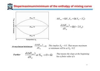
Sd at maximum, this corresponds to XB = 0.5
Further, the slope at XB →0 is infinite. That means
the entropy change is very high in a dilute solution
As mentioned earlier the total free energy after mixing
can be written as GGG ∆+=can be written as mixGGG ∆+= 0
where
]lnln[
0
BBAAmix
BAmix
mixmixmix
BBAA
XXXXRS
XXH
STHG
GXGXG
+−=∆
Ω=∆
∆−∆=∆
+=
So ∆Gmix can be written as ]lnln[ BBAABAmix XXXXRTXXG ++Ω=∆
]lnln[ BBAABABBAA XXXXRTXXGXGXG ++Ω++=
Following, total free energy of the system after mixing can be written as
52](https://image.slidesharecdn.com/phasetransformationsheattreatment-160429085624/85/Phase-Transformations-Heat-Treatment-Lecture-Notes-52-320.jpg)
![Free energy of mixing
We need to consider three situations for different kinds of enthalpy of mixing
Situation 1: Enthalpy of mixing is zero
mixGGG ∆+= 0
mixSTG ∆−= 0
]lnln[ BBAABBAA XXXXRTGXGX +++=
With the increase in temperature, -T∆Smix
will become even more negative.
The values of GA and GB also will decrease.
Following the slope Go might change since
GA and GB will change differently with
temperature.
54](https://image.slidesharecdn.com/phasetransformationsheattreatment-160429085624/85/Phase-Transformations-Heat-Treatment-Lecture-Notes-54-320.jpg)
![Situation 2: Enthalpy of mixing is negative
]lnln[ BBAABABBAA XXXXRTXXGXGXG ++Ω++=
Negative
∆Hmix
G0 -T∆Smix
Here both ∆Hmix and -T∆Smix are negative
Free energy of mixing
Here both ∆Hmix and -T∆Smix are negative
With increasing temperature G will become even
more negative.
Note that here also G0 may change the slope
because of change of GA and GB differently with
temperature.
55](https://image.slidesharecdn.com/phasetransformationsheattreatment-160429085624/85/Phase-Transformations-Heat-Treatment-Lecture-Notes-55-320.jpg)
![Free energy of mixing
Situation 3: Enthalpy of mixing is positive
]lnln[ BBAABABBAA XXXXRTXXGXGXG ++Ω++=
Positive ∆HmixG0
-T∆Smix
∆Hmix is positive but -T∆Smix is negative. At lower
temperature, in a certain mole fraction range the
absolute value of ∆Hmix could be higher than T∆Smix
so that G goes above the G line.so that G goes above the G0 line.
However to GA and GB, G will always be lower than
G0 , since ∆Hmix has a finite slope, where as ∆Smix
has infinite slope. The composition range, where G
is higher than G0 will depend on the temperature i.e.,
-T∆Smix
Because of this shape of the G, we see miscibility
gap in certain phase diagrams.
At higher temperature, when the absolute value of -
T∆Smix will be higher than ∆Hmix at all
compositions, G will be always lower than G0
56](https://image.slidesharecdn.com/phasetransformationsheattreatment-160429085624/85/Phase-Transformations-Heat-Treatment-Lecture-Notes-56-320.jpg)


![Concept of the chemical potential and the activity of elements
Let us consider an alloy of total X moles where it has XA mole of A and XB mole of B.
Note that x is much higher than 1 mole.
Now suppose we add small amounts of A and B in the system, keeping the ratio of XA : XB
the same, so that there is no change in overall composition.
So if we add four atoms of A, then we need to add six atoms of B to keep the overall
composition fixed. Following this manner, we can keep on adding A and B and will reach
to the situation when XA mole of A and XB mole of B are added and total added amount is
XA + XB = 1
Since previously we have considered that the total free energy of 1 mole of alloy afterSince previously we have considered that the total free energy of 1 mole of alloy after
mixing is G, then we can write
Previously, we derived
Further, we can write
BAAA XXG µµ +=
]lnln[ BBAABABBAA XXXXRTXXGXGXG ++Ω++=
22
BABABA XXXXXX +=
)ln()ln( 22
BABBBBAA XRTXGXXRTXGXG +Ω+++Ω+=
62](https://image.slidesharecdn.com/phasetransformationsheattreatment-160429085624/85/Phase-Transformations-Heat-Treatment-Lecture-Notes-62-320.jpg)


![Equilibrium vacancy concentration in a pure element
Further there will be change in configurational entropy considering the mixing of A and V
and can be expressed as (Note that we are considering XA + XV = 1
Total entropy of mixing
Total free energy in the presence of vacancies
)]1ln()1(ln[]lnln[ VVVVAAVVconfig XXXXRXXXXRS −−+−=+−=∆
)]1ln()1(ln[ VVVVVVmix XXXXRXSS −−+−∆=∆
(Total contribution from thermal and configurational entropy)
GGG A ∆+=
STHGA ∆−∆+=
{ })]1ln()1(ln[ VVVVVVVA XXXXRSTHXG −−+−∆−∆+=
Note here that G of element A when vacancies are
present decreases. So always there will be vacancies
present in materials. Further G decreases to a minimum
value and then increases with the further increase in
vacancy concentration. So, in equilibrium condition,
certain concentration of vacancies will be present,
which corresponds to Ge.
70](https://image.slidesharecdn.com/phasetransformationsheattreatment-160429085624/85/Phase-Transformations-Heat-Treatment-Lecture-Notes-70-320.jpg)


![Equilibrium concentration of interstitial atoms
Further, there will be two different types of contribution on entropy
Vibration of atoms A, next to interstitial atoms will change from normal mode of vibration
and will be more random and irregular because of distortion of the lattice
∆SI is the change of the entropy of one mole of atoms because of change in vibration pattern
From the crystal structure, we can say that for 2 solvent atoms there are 6 sites for
interstitial atoms. So if we consider that there are N0 numbers of A atoms then there will be
3N0 numbers of sites available for interstitial atoms.
In other sense, we can say that n atoms will randomly occupy in 3N sites available. So the
IIthermal SXS ∆=∆
In other sense, we can say that nI atoms will randomly occupy in 3N0 sites available. So the
configurational entropy can be written as
)3(!
!3
lnln
0
0
II
config
nNn
N
kwkS
−
==∆ Following Stirling’s approximation NNNN −= ln!ln
)]3ln()3(ln3ln3[ 0000 IIIIconfig nNnNnnNNkS −−−−=∆
−
−
−−=∆ )3ln(
3
ln3ln3 0
0
0
0
0 I
I
I
I
config nN
N
nN
n
N
n
NRS
74](https://image.slidesharecdn.com/phasetransformationsheattreatment-160429085624/85/Phase-Transformations-Heat-Treatment-Lecture-Notes-74-320.jpg)


![1. The specific heat of solid copper above 300 K is given by .
By how much does the entropy of copper increase on heating from 300 to 1358 K?
2. Draw the free energy temperature diagram for Fe up to 1600oC showing all the allotropic
forms.
3. From the thermodynamic principles show that the melting point of a nanocrystalline metal
would be different from that of bulk metal. Will the melting point be different if the
nanoparticle is embedded in another metal?
4. What is Clausius-Clapeyron equation? Apply it for the solidification of steels and gray cast
iron.
Questions?
-1-13
Kmole1028.664.22 JTCP
−
×+=
iron.
5. If the equilibrium concentration of vacancies in terms of mol fraction at 600 °C is 3x10⁻⁶
calculate the vacancy concentration at 800 °C. R = 8.314 J/mol.K
For aluminium ∆HV = 0.8 eV atom-1 and ∆SV/R = 2. Calculate the equilibrium vacancy
concentration at 660oC (Tm) at 25oC
6. Derive
7. Show that the free energy of a mixture of two phases in equilibrium in a binary system is
given by the point on the common tangent line that corresponds to that overall composition.
Show that the free energy of a mixture of phases of any other composition or a single phase
is higher.
]lnln[ BBAA
mix
Conf XXXXRS +−=∆
87](https://image.slidesharecdn.com/phasetransformationsheattreatment-160429085624/85/Phase-Transformations-Heat-Treatment-Lecture-Notes-87-320.jpg)


![Diffusional processes can be either steady-state or non-steady-state. These two types of
diffusion processes are distinguished by use of a parameter called flux.
It is defined as net number of atoms crossing a unit area perpendicular to a given direction
per unit time. For steady-state diffusion, flux is constant with time, whereas for
non-steady-state diffusion, flux varies with time.
A schematic view of concentration gradient with distance for both steady-state and non-
steady-state diffusion processes are shown below.
Flux (J) (restricted definition) → Flow / area / time [Atoms / m2 / s]
steady and non-steady state diffusion
Concentration→
Distance, x →
Steady state diffusion
D ≠ f(c)
t1
Non-Steady state diffusion
Concentration→
Distance, x →
t2
t3
D = f(c)
Flux (J) (restricted definition) → Flow / area / time [Atoms / m2 / s]
Steady state
J ≠ f(x,t)
Non-steady state
J = f(x,t)
C1
C1
C2
C2
111](https://image.slidesharecdn.com/phasetransformationsheattreatment-160429085624/85/Phase-Transformations-Heat-Treatment-Lecture-Notes-111-320.jpg)


![↑ ∆Hfusion
↓ ∆Hd ≈∝ Log [Viscosity (η)]
Crystallization favoured by
High → (10-15) kJ / mole
Low → (1-10) Poise
Metals
Thermodynamic
Kinetic
2
* 1
fusionH
G
∆
∝∆
Mechanism of Crystallization
Enthalpy of activation for
diffusion across the interface
Difficult to amorphize metals
Very fast cooling rates ~106 K/s are used for the amorphization of alloys
→ splat cooling, melt-spinning.
168](https://image.slidesharecdn.com/phasetransformationsheattreatment-160429085624/85/Phase-Transformations-Heat-Treatment-Lecture-Notes-168-320.jpg)


![Homogenous Nucleation Rate
The process of nucleation (of a crystal from a liquid melt, below Tm
Bulk) we have described
so far is a dynamic one. Various atomic configurations are being explored in the liquid
state - some of which resemble the stable crystalline order. Some of these ‘crystallites’ are
of a critical size r*∆T for a given undercooling (∆T). These crystallites can grow to
transform the melt to a solid→by becoming supercritical. Crystallites smaller than r*
(embryos) tend to ‘dissolve’.
As the whole process is dynamic, we need to describe the process in terms of ‘rate’ →the
nucleation rate [dN/dt ≡ number of nucleation events/time].
Also, true nucleation is the rate at which crystallites become supercritical. To find theAlso, true nucleation is the rate at which crystallites become supercritical. To find the
nucleation rate we have to find the number of critical sized crystallites (N*) and multiply it
by the frequency/rate at which they become supercritical.
If the total number of particles (which can act like potential nucleation sites - in
homogenous nucleation for now) is Nt , then the number of critical sized particles given by
an Arrhenius type function with a activation barrier of ∆G*.
∆
−
=
kT
G
t eNN
*
*
188](https://image.slidesharecdn.com/phasetransformationsheattreatment-160429085624/85/Phase-Transformations-Heat-Treatment-Lecture-Notes-188-320.jpg)


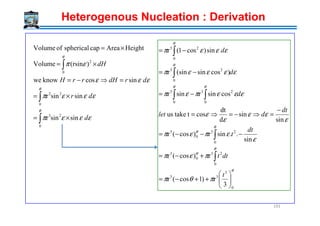
![]coscos32[
3
3
1coscos33
)1(cos
3
r
)cos1(r
)0cos(cos
3
r
)cos1(r
3
3
3
3
3
3
3
33
3
3
θθ
π
θθ
π
θ
π
θπ
θ
π
θπ
+−=
−+−
=
−+−=
−+−=
r
r
Heterogenous Nucleation : Derivation
γαβ
γαδ
αααα
ββββ
δδδδ
γβδ
θθθθ
βδαδ
γ
γγ
θ
−
=Cos
194
3
2.EqCos
Cos
⇒
−
=
−=
αβ
βδαδ
βδαδαβ
γ
γγ
θ
γγθγ
αβγ
θ =Cos
Surface tension force balance
θγγγ
γγθπθπγθθ
π
αβαδβδ
αδβδαβ
cos
)(sin)cos1(2]coscos32[
3
2223
3
−=−
−+−+∆+−=∆
put
rrG
r
G V](https://image.slidesharecdn.com/phasetransformationsheattreatment-160429085624/85/Phase-Transformations-Heat-Treatment-Lecture-Notes-194-320.jpg)
![4
]coscos32[
4
4
]coscos32[
3
4
)cos)cos1(cos22(
4
]coscos32[
3
4
)cossincos22(
4
]coscos32[
3
4
cossin)cos1(2]coscos32[
3
3
2
33
22
33
22
33
2223
3
θθ
γπ
θθπ
θθθγπ
θθπ
θθγπ
θθπ
θθπγθπγθθ
π
αβ
αβ
αβ
αβαβ
rG
r
rG
r
rG
r
rrG
r
V
V
V
V
+−
+∆
+−
=
−−−+∆
+−
=
−−+∆
+−
=
−−+∆+−=
Heterogenous Nucleation : Derivation
195
)()(*).(*)(
)(.
4
]coscos32[
)()(]4
3
4
[
]4
3
4
[
4
]coscos32[
443
**
3
2
3
2
33
θθ
θ
θθ
θθγπ
π
γπ
πθθ
αβ
αβ
fGfrGrGG
fGG
fwherefrG
r
rG
r
HomoHetero HomoHetero
HomoHetero
V
V
∆=∆=∆=∆
∆=∆
+−
=→+∆=
+∆
+−
=
Nucleation barrier can be significantly lower for heterogeneous nucleation due to wetting
angle affecting the shape of the nucles](https://image.slidesharecdn.com/phasetransformationsheattreatment-160429085624/85/Phase-Transformations-Heat-Treatment-Lecture-Notes-195-320.jpg)


![6. Assume for the solidification of nickel that nucleation is homogeneous, and the number of
stable nuclei is 106 nuclei per cubic meter. Calculate the critical radius and the number of
stable nuclei that exist at the following degrees of supercooling: 200 K and 300 K. and
What is significant about the magnitudes of these critical radii and the numbers of stable
nuclei? [rNi – 0.255 J/m2, ΔHf = -2.53×10⁹ J/m3, Super cooling value for Ni = 319oC]
7. Calculate the homogeneous nucleation rate in liquid copper at under coolings of 180, 200,
and 220K, using the given data: L =1.88×10⁹ J m-3, Tm = 1356K, γsL = 0.177 J m-2, f0 = 1011
s-1, C0 = 6×1028 atoms m-3, k = 1.38×1
8. Explain the concept constitutional Supercooling. When does this take place? And explain
Questions?
8. Explain the concept constitutional Supercooling. When does this take place? And explain
dendritic formation
9. The surface energy of pure metal liquid , γ, is 600 dynes/ cm; The volume of an atom of this
metal in the liquid is 2.7×10⁻²⁵cm3; and the free-energy difference between an atom in the
vapor and liquid , ΔGvl, is -2.37J. Under these conditions, what would be the critical radius
of a droplet, r0 in nm and the free energy of the droplet, ΔGr0, in J?
10. Write a short note on ‘Grwoth of a pure solid’ ?
11. Differentiate between Homogeneous and Heterogeneous nucleation? In which case
nucleation rate will be high? Why.
12. Explain the effect of undercooling on Nucleation rate, growth rate, r* and G*? And what is
the glass transition temperature. And how it is related to undercooling.
204](https://image.slidesharecdn.com/phasetransformationsheattreatment-160429085624/85/Phase-Transformations-Heat-Treatment-Lecture-Notes-204-320.jpg)

![16. Estimate entropy change during solidification of the following elements and comment on the
nature of the interface between solidifying crystal and liquid. The latent heat and melting point
are given with brackets. (a) Al [10.67kJ/mole, 660C] (b) Si [46.44kJ/mole, 1414⁰C]
17. What is partition coefficient? Derive Scheil equation for solidification of binary alloys. State the
assumptions made during its derivation. What is the composition of the last solid that forms
during solidification of a terminal solid solution of a binary eutectic system?
18. Estimate the temperature gradient that is to be maintained within solid aluminum so that the
planar solidification front moves into liquid aluminum maintained at its melting point at a
velocity of 0.001m/s. Given thermal conductivity of aluminum = 225 W/mK, latent heat of fusion
= 398 KJ/kg and density = 2700kg/m3 .
Questions?
= 398 KJ/kg and density = 2700kg/m3 .
19. In cobalt, a coherent interface forms during HCP to FCC transformation. The lattice parameter of
the FCC phase is 3.56 Ao. The distance between nearest neighbours along a close packed
direction in the basal plane of the HCP phase is 2.507Ao. show that the misfit to be
accommodated by coherency strains is small.
20. Suppose that an iron specimen containing 0.09 atomic percent carbon is equilibriated at 720°C
(993 K) and then rapidly quenched to 300°C (573 K). Determine the length of the time needed for
one side of a plate shaped carbide precipitate to grow out by 103 nm.
p) How wide a layer of the matrix next to a plate would have its carbon concentration lowered
from 0.09 percent carbon to that corresponding to nα
e to form a layer of cementite 103 nm
thick?
q) How long would it take to increase one side of the plate by 10 nm? 206](https://image.slidesharecdn.com/phasetransformationsheattreatment-160429085624/85/Phase-Transformations-Heat-Treatment-Lecture-Notes-206-320.jpg)


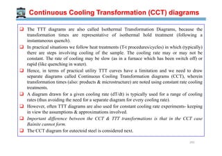
![Temperature→
Peritectic
L + δ → γ
Eutectic
L → γ + Fe3C
Liquid (L)
L + γγγγ
γγγγ (Austenite)
[γγγγ(Austenite) + Fe3C(Cementite)] = Ledeburite
δδδδ (Ferrite)
1493ºC
1147ºC
2.11
L + Fe3C
Hypo Eutectic
0.16
Hyper Eutectic
0.1 0.51
δδδδ+ γγγγ
910ºC
Fe-Fe3C metastable phase diagram
% Carbon →
Temperature
Fe Fe3C
6.7
4.3
0.8
Eutectoid
γ → α + Fe3C
αααα (Ferrite)
[γγγγ(Austenite) + Fe3C(Cementite)] = Ledeburite
723ºC
0.025 %C
[αααα (Ferrite) + Fe3C (Cementite)] = Pearlite
Hypo
Eutectoid
Hyper
Eutectoid
0.008
Steels Cast Irons
212](https://image.slidesharecdn.com/phasetransformationsheattreatment-160429085624/85/Phase-Transformations-Heat-Treatment-Lecture-Notes-212-320.jpg)


![Phase changes that occur upon passing from the γ
region into the α+ Fe3C phase field.
Consider, for example, an alloy of eutectoid
composition (0.8%C) as it is cooled from a temperature
within the γ phase region, say 800ºC – that is,
beginning at point ‘a’ in figure and moving down
vertical xx’. Initially the alloy is composed entirely of
the austenite phase having composition 0.8 wt.% C and
then transformed to α+ Fe3C [pearlite]
The microstructure for this eutectoid steel that is slowly
Eutectoid Reaction
The microstructure for this eutectoid steel that is slowly
cooled through eutectoid temperature consists of
alternating layers or lamellae of the two phases α and
Fe3C
The pearlite exists as grains, often termed “colonies”;
within each colony the layers are oriented in essentially
the same direction, which varies from one colony to
other.
The thick light layers are the ferrite phase, and the
cementite phase appears as thin lamellae most of which
appear dark.
229](https://image.slidesharecdn.com/phasetransformationsheattreatment-160429085624/85/Phase-Transformations-Heat-Treatment-Lecture-Notes-229-320.jpg)


![Transformation Rate
rate)Growthrate,onf(NucleatiratetionTransforma =∆T
Tm
U
),( UIf
dt
dX
T ==
β
Maximum of growth rate usually
at higher temperature than
maximum of nucleation rate
I, U, Tr → [rate ⇒ Sec-1 ]
T(K)→Increasing∆
0
T
I
267](https://image.slidesharecdn.com/phasetransformationsheattreatment-160429085624/85/Phase-Transformations-Heat-Treatment-Lecture-Notes-267-320.jpg)

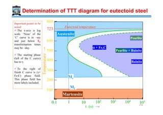
![From ‘Rate’ to ‘time’ : The Origin of TTT diagrams
The transformation rate curve (Tr -T plot) has hidden in it the I-T and U-T curves.
An alternate way of plotting the Transformation rate (Tr ) curve is to plot Transformation
time (Tt) [i.e. go from frequency domain to time domain]. Such a plot is called the Time-
Temperature-Transformation diagram (TTT diagram).
High rates correspond to short times and vice-versa. Zero rate implies ∞ time (no
transformation).
This Tt -T plot looks like the ‘C’ alphabet and is often called the ‘C-curve. The minimum
time part is called the nose of the curve.
Tr (rate ⇒ sec−1) →
Tr
Tm
0
Replot
( , )Rate f T t=
Tt (rate ⇒ sec−1) →
T(K)→
Tm
0
Time for transformation
Small driving
force for nucleation
Sluggish
growth
Nose of the ‘C-curve’
Tt
T(K)→
269](https://image.slidesharecdn.com/phasetransformationsheattreatment-160429085624/85/Phase-Transformations-Heat-Treatment-Lecture-Notes-269-320.jpg)
![Understanding the TTT diagram
Though we are labeling the transformation temperature Tm , it represents other
transformations, in addition to melting.
Clearly the Tt function is not monotonic in undercooling. At Tm it takes infinite time for
transformation.
Till T3 the time for transformation decreases (with undercooling) [i.e. T3 < T2 < T1 ]
→due to small driving force for nucleation.
After T3 (the minimum) the time for transformation increases [i.e. T3 < T4 < T5]→due
to sluggish growth.
The diagram is called the TTT diagram because it
plots the time required for transformation if we hold
the sample at fixed temperature (say T1) or fixed
undercooling (∆T1). The time taken at T1 is t1.
To plot these diagrams we have to isothermally hold
at various undercoolings and note the transformation
time. I.e. instantaneous quench followed by
isothermal hold.
Hence, these diagrams are also called Isothermal
Transformation Diagrams. Similar curves can be
drawn for α→β (solid state) transformation. 270](https://image.slidesharecdn.com/phasetransformationsheattreatment-160429085624/85/Phase-Transformations-Heat-Treatment-Lecture-Notes-270-320.jpg)


![Parent phase has a fixed number of nucleation sites Nn per unit volume (and these sites are
exhausted in a very short period of time
Growth rate (U = dr/dt) constant and isotropic (as spherical particles) till particles impinge
on one another.
At time t the particle that nucleated at t = 0 will have a radius r = Ut
Between time t = t and t = t + dt the radius increases by dr = Udt
The corresponding volume increase dV = 4πr2 dr
Without impingement, the transformed volume fraction (f) (the extended transformed
volume fraction) of particles that nucleated between t = t and t = t + dt is:
Derivation of f(T,t) : Avrami Model
volume fraction) of particles that nucleated between t = t and t = t + dt is:
This fraction (f) has to be corrected for impingement. The corrected transformed volume
fraction (X) is lower than f by a factor (1−X) as contribution to transformed volume fraction
comes from untransformed regions only:
Based on the assumptions note that the growth rate is not part of the equation →it is only
the number of nuclei.
( ) [ ] ( )2 3 22
4 4 4n n nr Utf N N N U t dtdr Udtπ π π= = =
1
dX
f
X
=
−
⇒ 3 2
4
1
n
dX
N U t dt
X
π=
−
3 2
0 0
4
1
X t t
n
t
dX
N U t dt
X
π
=
=
=
−∫ ∫⇒
3 3
n4π N U t
3
βX 1 e
−
= −
276](https://image.slidesharecdn.com/phasetransformationsheattreatment-160429085624/85/Phase-Transformations-Heat-Treatment-Lecture-Notes-276-320.jpg)
![Derivation of f(T,t): Johnson-Mehl Model
Parent phase completely transforms to product phase (α → β)
Homogenous Nucleation rate of β in untransformed volume is constant (I)
Growth rate (U = dr/dt) constant and isotropic (as spherical particles) till particles impinge
on one another
At time t the particle that nucleated at t = 0 will have a radius r = Ut
The particle which nucleated at t = τ will have a radius r = U(t − τ)
Number of nuclei formed between time t = τ and t = τ + dτ → Idτ
Without impingement, the transformed volume fraction (f) (called the extended transformedWithout impingement, the transformed volume fraction (f) (called the extended transformed
volume fraction) of particles that nucleated between t = τ and t = τ + dτ is:
This fraction (f) has to be corrected for impingement. The corrected transformed volume
fraction (X) is lower than f by a factor (1−X) as contribution to transformed volume fraction
comes from untransformed regions only:
1
dX
f
X
=
−
⇒ ( ) [ ] ( )
334 4
1 3 3
( )Idr U
dX
X
t Idπτπ τ τ= = −
−
( ) [ ] ( )
334 4
3 3
( )r U t If Id dτπ τ τπ −= =
277](https://image.slidesharecdn.com/phasetransformationsheattreatment-160429085624/85/Phase-Transformations-Heat-Treatment-Lecture-Notes-277-320.jpg)
![Xβ→
1.0
0.5
Xβ→
1.0
0.5
[ ] ( )
0 0
3
(
4
1 3
)
X t
U t Id
dX
X
τ
τ
ττπ
=
=
=
−
−∫ ∫
−
−=
3
tUIπ
β
43
e1X
For a isothermal transformation
Derivation of f(T,t): Johnson-Mehl Model
t →
0
t →
0
3
π I U
is a constant during isothermal transformation
3
→
Note that Xβ is both a function of I and
U. I & U are assumed constant
278](https://image.slidesharecdn.com/phasetransformationsheattreatment-160429085624/85/Phase-Transformations-Heat-Treatment-Lecture-Notes-278-320.jpg)


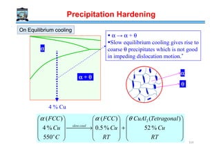


![10 ,100nmthick nmdiameter
Distorted FCCDistorted FCC
Unitcell composition
Al6Cu2 = Al3Cu
Become incoherent as ppt. grows
'θ
''θ
αθ
)001()001( ''
αθ
]100[]100[ ''
αθ
)001()001( '
TetragonalTetragonal
Precipitation Hardening
Body CenteredBody Centered
TetragonalTetragonal
α
θ
αθ
]100[]100[ '
TetragonalTetragonal
Unitcell composition
Al4Cu2 = Al2Cu
Unitcell composition
Al8Cu4 = Al2Cu
320](https://image.slidesharecdn.com/phasetransformationsheattreatment-160429085624/85/Phase-Transformations-Heat-Treatment-Lecture-Notes-320-320.jpg)


![Rate of coarsening
In superalloys, Strength obtained by fine dispersion of γ’ [ordered FCC Ni3(TiAl)]
precipitate in FCC Ni rich matrix
Matrix (Ni SS)/ γ’ matrix is fully coherent [low interfacial energy γ = 30 mJ/m2]
Misfit = f(composition) → varies between 0% and 0.2%
Creep rupture life increases when the misfit is 0% rather than 0.2%
Low γγγγ
Low Xe
ThO2 dispersion in W (or Ni) (Fine oxide dispersion in a metal matrix)
Oxides are insoluble in metals
Stability of these microstructures at high temperatures due to low value of Xe
The term DγXe has a low value
ThO2 dispersion in W (or Ni) (Fine oxide dispersion in a metal matrix)
Cementite dispersions in tempered steel coarsen due to high D of interstitial C
If a substitutional alloying element is added which segregates to the carbide → rate of coarsening
↓ due to low D for the substitutional element
Low D
334](https://image.slidesharecdn.com/phasetransformationsheattreatment-160429085624/85/Phase-Transformations-Heat-Treatment-Lecture-Notes-334-320.jpg)


![Temperature→
Peritectic
L + δ → γ
Eutectic
L → γ + Fe3C
Liquid (L)
L + γγγγ
γγγγ (Austenite)
[γγγγ(Austenite) + Fe C(Cementite)] = Ledeburite
δδδδ (Ferrite)
1493ºC
1147ºC
2.11
L + Fe3C
Hypo Eutectic
0.16
Hyper Eutectic
0.1 0.51
δδδδ+ γγγγ
910ºC
Eutectoid Transformation in Fe-Fe3C phase diagram
% Carbon →
Temperature
Fe Fe3C
6.7
4.3
0.8
Eutectoid
γ → α + Fe3C
αααα (Ferrite)
[γγγγ(Austenite) + Fe3C(Cementite)] = Ledeburite
723ºC
0.025 %C
[αααα (Ferrite) + Fe3C (Cementite)] = Pearlite
Hypo
Eutectoid
Hyper
Eutectoid
0.008
Iron – Cementite Phase Diagram
Steels Cast Irons
344](https://image.slidesharecdn.com/phasetransformationsheattreatment-160429085624/85/Phase-Transformations-Heat-Treatment-Lecture-Notes-344-320.jpg)


![Time and Temperature relationship in Tempering
For a given steel, a heat treater might like to choose some convenient tempering time, say
over night, otherwise different than 1 hour, and thus, wants to calculate the exact
temperature required to achieve the constant hardness.
Hollomon and Jaffe’s “tempering parameter” may be used for this purpose as it relates the
hardness, tempering temperature and tempering time. For a thermally activated process, the
usual rate equation is :
Where, t is the time of tempering to develop a given hardness, and Q is the ‘empirical
activation energy’ . ‘Q’ is not constant in the complex tempering processes but varies with
RTQ
Ae
t
Rate /1 −
==
activation energy’ . ‘Q’ is not constant in the complex tempering processes but varies with
hardness. Thus, hardness was assumed to be a function of time and temperature:
Interestingly, is a constant, and let it be t0. Equating activation energies of eq (1)
and (2) gives,
As t0 constant then
Where, C is a constant, whose value depends on the composition of austenite. The single
parameter which expresses two variables time and the temperature i.e., T (C + ln t) is called
the Hollomon and Jaffe tempering parameter. (hardness in vickers is preferable)
][ / RTQ
tefH −
=
][ / RTQ
te−
[ ] )(lnln 0 HfttTQ =−=
[ ])ln( tCTfH +=
436](https://image.slidesharecdn.com/phasetransformationsheattreatment-160429085624/85/Phase-Transformations-Heat-Treatment-Lecture-Notes-436-320.jpg)


![Process Variable H Value
Air No agitation 0.02
Oil quench No agitation 0.2
" Slight agitation 0.35
" Good agitation 0.5
" Vigorous agitation 0.7
Water quench No agitation 1.0
" Vigorous agitation 1.5
Brine quench
No agitation 2.0
Severity of Quench as indicated by the heat
transfer equivalent H
If the increase in rate of heat
conduction is greater than the
decrease due to persistence of the
vapor film, the net result will be an
increase in the actual cooling rate.
However if the reverse is true, then the
result will be decrease in cooling rate.
Severity of Quenching media
Brine quench
(saturated Salt water)
No agitation 2.0
" Vigorous agitation 5.0
Ideal quench ∞
Note that apart from the nature of the quenching medium, the vigorousness of the shake determines the
severity of the quench. When a hot solid is put into a liquid medium, gas bubbles form on the surface of
the solid (interface with medium). As gas has a poor conductivity the quenching rate is reduced.
Providing agitation (shaking the solid in the liquid) helps in bringing the liquid medium in direct
contact with the solid; thus improving the heat transfer (and the cooling rate). The H value/index
compares the relative ability of various media (gases and liquids) to cool a hot solid. Ideal quench is a
conceptual idea with a heat transfer factor of ∞ (⇒ H = ∞)
1
[ ]
f
H m
K
−
=
f → heat transfer factor
K → Thermal conductivity
467](https://image.slidesharecdn.com/phasetransformationsheattreatment-160429085624/85/Phase-Transformations-Heat-Treatment-Lecture-Notes-467-320.jpg)


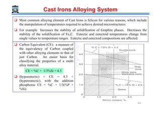


![Fe-C-Si + (Mn, P, S)
→ Invariant lines become invariant regions in phase diagram
< 0.1% → retards graphitization; ↑ size of Graphite flakes
< 1.25% → Inhibits graphitization
∈ [2.4% (for good castability), 3.8 (for OK mechanical propeties)]
Grey Cast Iron
→ Invariant lines become invariant regions in phase diagram
Si ∈ (1.2, 3.5) → C as Graphite flakes in microstructure (Ferrite matrix)
3 3 3L ( ) ( )
Ledeburite Pearlite
Fe C Fe C Fe Cγ α→ + → + +
14243 14243
Si eutectoidC↑⇒
suuuuuuuu
↑ volume during solidification ⇒ better castability
Most of the ‘P’ combines with the iron to form iron phosphide (Fe3P).This iron
phosphide forms a ternary eutectic known as steadite, contains cementite and
austenite (at room temperature pearlite).
501](https://image.slidesharecdn.com/phasetransformationsheattreatment-160429085624/85/Phase-Transformations-Heat-Treatment-Lecture-Notes-501-320.jpg)


![Excellent resistance to oxidation at high temperatures
High Cr Cast Irons are of 3 types:
12-28 % Cr matrix of Martensite + dispersed carbide
29-34 % Cr matrix of Ferrite + dispersion of alloy carbides
[(Cr,Fe)23C6, (Cr,Fe)7C3]
15-30 % Cr + 10-15 % Ni stable γ + carbides [(Cr,Fe)23C6, (Cr,Fe)7C3]
Ni stabilizes Austenite structure
Chromium addition (12-35 wt %)
Ni stabilizes Austenite structure
29.3% Cr, 2.95% C 519](https://image.slidesharecdn.com/phasetransformationsheattreatment-160429085624/85/Phase-Transformations-Heat-Treatment-Lecture-Notes-519-320.jpg)


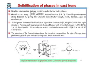
The document outlines a course on phase transformations and heat treatment in metallic materials, aiming to enhance understanding of their microstructures and properties. It covers thermodynamics of phase transformations, heat treatment processes, and introduces important concepts such as diffusional and diffusionless transformations. The course includes various chapters discussing fundamental principles, classification of transformations, and provides references for further study.


![[S.L._Kakani]_Material_Science_(New_Age_Pub.,_2006(BookSee.org).pdf](https://cdn.slidesharecdn.com/ss_thumbnails/s-230301071329-4f25d7e9-thumbnail.jpg?width=640&height=640&fit=bounds)


