Downloaded 59 times

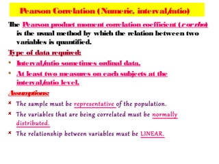
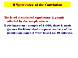
nzXzYr ∑=
Where:
ZX= the z-score of variable X
ZY= the z-score of variable Y
N= number of observations](https://image.slidesharecdn.com/correlation2-140504133244-phpapp02/85/Linear-Correlation-8-320.jpg)
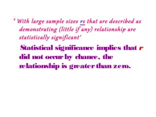
nzXzYr ∑=
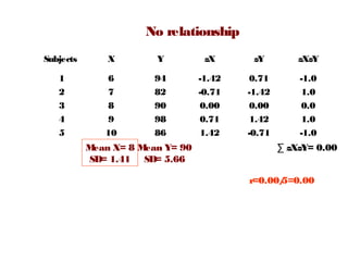
A five subjects took a quiz X, on which the scores ranged from
6to 10 and an examination Y, on which the scores ranged form
82to 98.
Calculate r and determine the pattern of correlation?](https://image.slidesharecdn.com/correlation2-140504133244-phpapp02/85/Linear-Correlation-15-320.jpg)
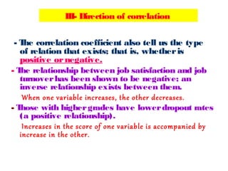
nzXzYr ∑=](https://image.slidesharecdn.com/correlation2-140504133244-phpapp02/85/Linear-Correlation-16-320.jpg)
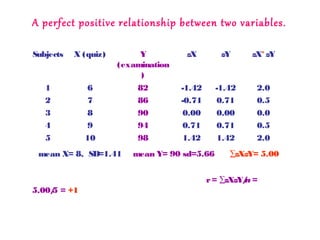
nzXzYr ∑= - =5.0/5-=1.0](https://image.slidesharecdn.com/correlation2-140504133244-phpapp02/85/Linear-Correlation-19-320.jpg)
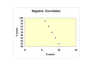
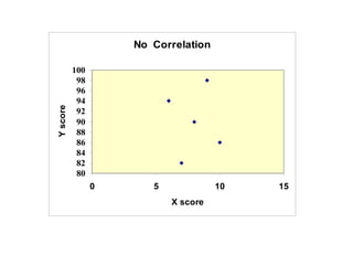
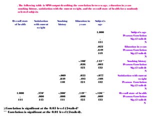
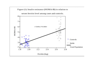
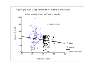

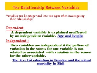
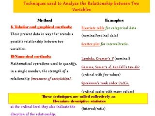
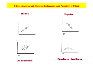
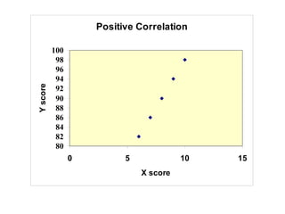
The document discusses the concept of correlation between variables, categorizing them into dependent and independent types. It details various methods for analyzing relationships, including tabular, graphical, and numerical techniques, and explains how to interpret correlation coefficients and statistical significance. Examples are provided to illustrate correlation calculation and relationships in data, including positive, negative, and no correlation scenarios.