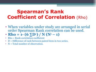
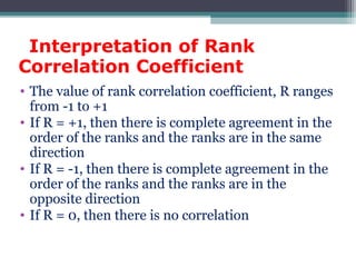
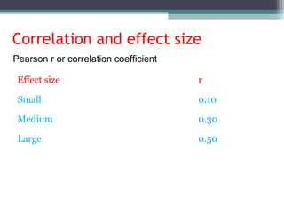
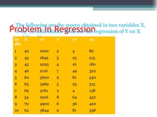
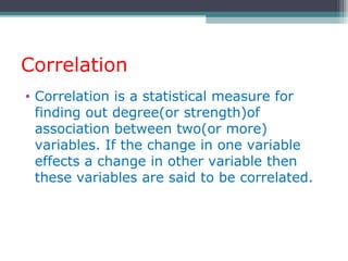
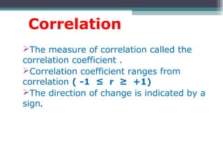
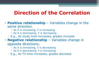
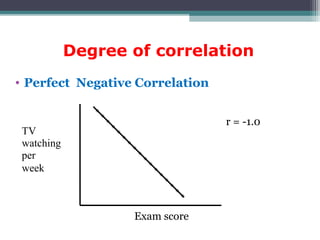
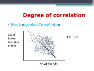
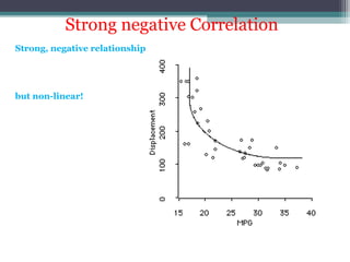
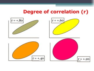
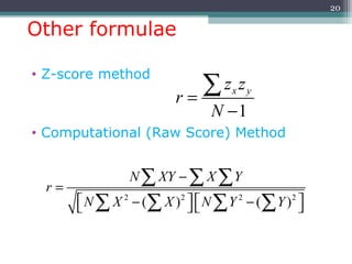
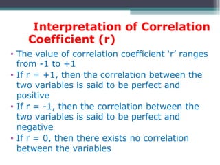
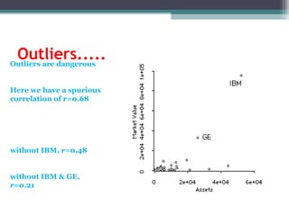
Correlation is a statistical measure of the degree of association between two or more variables. The correlation coefficient ranges from -1 to +1, with -1 indicating a perfect negative correlation, 0 indicating no correlation, and +1 indicating a perfect positive correlation. Correlation does not necessarily imply causation - two variables can be correlated without one causing changes in the other. There are different types of correlation coefficients that can be used depending on the type and scale of the variables, such as Pearson's correlation coefficient for continuous variables or Spearman's rank correlation coefficient for ordinal variables.

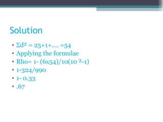
![Solution
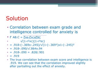
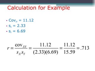
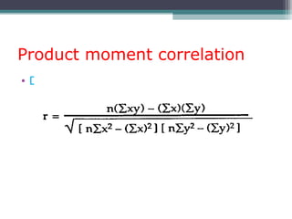
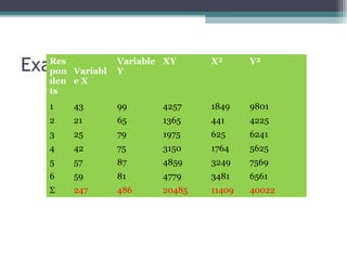
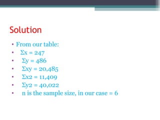
• = 6(20,485) – (247 × 486)
√[6(11,409) – 247²] × [6(40,022) – 486²]
• =0.5298](https://image.slidesharecdn.com/correlationandregression-190615193717/85/Correlation-and-regression-30-320.jpg)